Now that we rejected the hypotheses of independence, the next step is to obtain estimates of canonical correlation.
The estimated canonical correlations are found at the top of page 1 in the SAS output as shown below:
Canonical Correlation Analysis
| Canonical Correlation |
Adjusted Canonical Correlation |
Approximate Standard Error |
Squared Canonical Correlation |
|
|---|---|---|---|---|
| 1 | 0.994483 | 0.994021 | 0.001572 | 0.988996 |
| 2 | 0.878107 | 0.872097 | 0.032704 | 0.771071 |
| 3 | 0.383606 | 0.366795 | 0.121835 | 0.147153 |
The squared values of the canonical variate pairs, found in the last column, can be interpreted much in the same way as \(r^{2}\) values are interpreted.
We see that 98.9% of the variation in \(U_{1}\) is explained by the variation in \(V_{1}\), and 77.11% of the variation in \(U_{2}\) is explained by \(V_{2}\), but only 14.72% of the variation in \(U_{3}\) is explained by \(V_{3}\). These first two are very high canonical correlations and suggest that only the first two canonical correlations are important.
One can actually see this from the plots that SAS generates. The first canonical variate for sales is plotted against the first canonical variate for scores in the scatter plot for the first canonical variate pair:
Canonical Correlation Analysis - Sales Data
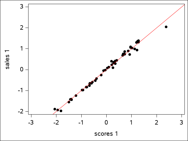
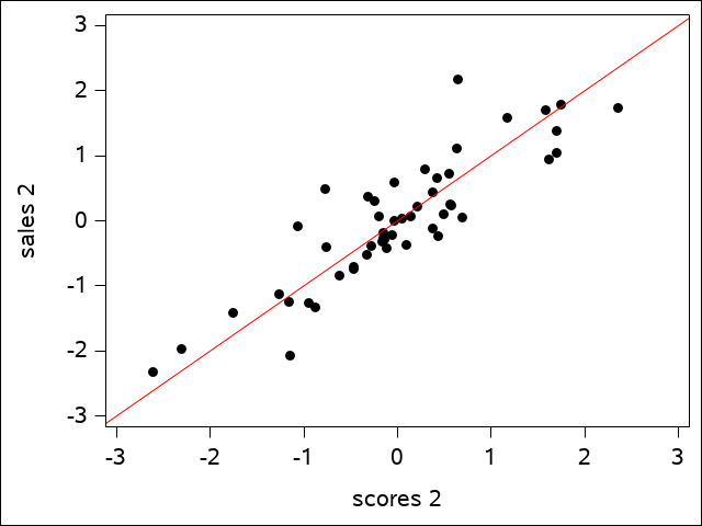
The regression line shows how well the data fits. The plot of the second canonical variate pair is a bit more scattered, but is still a reasonably good fit:
Canonical Correlation Analysis - Sales Data
A plot of the third pair would show little of the same kind of fit. We may refer to only the first two canonical variate pairs from this point on based on the observation that the third squared canonical correlation value is so small.