The next step of cluster analysis is to describe the identified clusters.
The SAS program shows how this is implemented.
Download the SAS Program here: wood1.sas
Notice that in the cluster procedure, we created a new SAS dataset called clust1.
- This contains the information required by the tree procedure to draw the tree diagram.
In the tree procedure, we chose to investigate 6 clusters with ncluster=6.
- A new SAS dataset called clust2 is output with the id numbers of each site and the cluster that site belongs stored in a new variable called a cluster.
- We need to merge this back with the original data to describe the characteristics of each of the 6 clusters.
Now an Analysis of Variance for each species is carried out with a class statement for the grouping variable, cluster.
- We also include the means statement to get the cluster means.
Performing a cluster analysis, part 2
To perform cluster analysis with follow-up ANOVA on clusters:
- Open the ‘wood’ data set in a new worksheet.
- Stat > Multivariate > Cluster Observations
- Highlight and select the variables to use in the clustering. For this example, the following variables are selected (13 total): carcar, corflo, faggra, ileopa, liqsty, maggra, nyssyl, ostvir, oxyarb, pingla, quenig, quemic, symtin.
- Choose Complete as the Linkage and Euclidean as the Distance.
- Choose Show dendrogram, and under Customize, choose Distance for Y-Axis.
- Under Storage, enter c34 (or the name of any blank column in the worksheet) in the Cluster membership column.
- Choose OK, and OK again. In addition to the session window results, the cluster assignments are stored in the c34 column. We relabel this column as ‘cluster’ for the steps below.
- Stat > ANOVA > One-way
- Highlight and select any one of the variables used in the original clustering (in this example, we use carcar) to move it to the Response window.
- Highlight and select cluster to move it to the Factor window.
- Choose OK. The results, including the F statistic, are shown in the session window.
Analysis
We perform an analysis of variance for each of the tree species, comparing the means of the species across clusters. The Bonferroni method is applied to control the experiment-wise error rate. This means that we will reject the null hypothesis of equal means among clusters at level \(\alpha\) if the p-value is less than \(\alpha/ p\). Here, \(p = 13\) so for an \(\alpha = 0.05\) level test, we reject the null hypothesis of equality of cluster means if the p-value is less than \(0.05/13\) or \(0.003846\).
Here is the output for the species carcar.
| Pr > F | |||||
|---|---|---|---|---|---|
| Model | 5 | 4340.834339 | 868.166868 | 62.94 | < 0.0001 |
| Error | 66 | 910.443439 | 13.794598 | ||
| Corrected Total | 71 | 5251.277778 | |||
| R-Square | Coeff Var | Root MSE | carcar Mean |
|---|---|---|---|
| 0.826624 | 44.71836 | 3.714108 | 8.305556 |
| Source | DF | Type I SS | Mean Square | F Value | Pr > F |
|---|---|---|---|---|---|
| CLUSTER | 5 | 4340.834339 | 868.166868 | 62.94 | < 0.0001 |
| Source | DF | Type III SS | Mean Square | F Value | Pr > F |
|---|---|---|---|---|---|
| CLUSTER | 5 | 4340.834339 | 868.166868 | 62.94 | < 0.0001 |
We collected the results of the individual species ANOVAs in the table below. The species names in boldface indicate significant results suggesting that there was significant variation among the clusters for that particular species.
| Code | Species | F | p-value |
|---|---|---|---|
| carcar | Ironwood | 62.94 | < 0.0001 |
| corflo | Dogwood | 1.55 | 0.1870 |
| faggra | Beech | 7.11 | < 0.0001 |
| ileopa | Holly | 3.42 | 0.0082 |
| liqsty | Sweetgum | 5.87 | 0.0002 |
| maggra | Magnolia | 3.97 | 0.0033 |
| nyssyl | Blackgum | 1.66 | 0.1567 |
| ostvir | Blue Beech | 17.70 | < 0.0001 |
| oxyarb | Sourwood | 1.42 | 0.2294 |
| pingla | Spruce Pine | 0.43 | 0.8244 |
| quenig | Water Oak | 2.23 | 0.0612 |
| quemic | Swamp Chestnut Oak | 4.12 | 0.0026 |
| symtin | Horse Sugar | 75.57 | < 0.0001 |
d.f. = 5, 66
The results indicate that there are significant differences among clusters for ironwood, beech, sweetgum, magnolia, blue beech, swamp chestnut oak, and horse sugar.
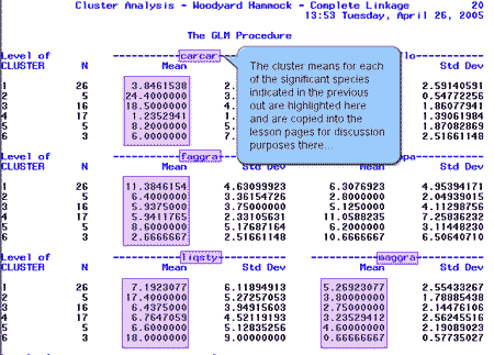
Next, SAS computed the cluster means for each of the species. Here is a sample of the output with a couple of significant species highlighted.

We collected the cluster means for each of the significant species indicated above and placed the values in the table below:
| Code | Cluster | |||||
|---|---|---|---|---|---|---|
| 1 | 2 | 3 | 4 | 5 | 6 | |
| carcar | 3.8 | 24.4 | 18.5 | 1.2 | 8.2 | 6.0 |
| faggra | 11.4 | 6.4 | 5.9 | 5.9 | 8.6 | 2.7 |
| liqsty | 7.2 | 17.4 | 6.4 | 6.8 | 6.6 | 18.0 |
| maggra | 5.3 | 3.8 | 2.8 | 3.2 | 4.6 | 0.7 |
| ostvir | 4.3 | 2.8 | 2.9 | 13.8 | 3.6 | 14.0 |
| quemic | 5.3 | 5.2 | 9.4 | 4.1 | 7.0 | 2.3 |
| symtin | 0.9 | 0.0 | 0.7 | 2.0 | 18.0 | 20.0 |
The boldface values highlight the clusters where each species is abundant. For example, carcar (ironwood) is abundant in clusters 2 and 3. This operation is carried out across the rows of the table.
Each cluster is then characterized by the species that are highlighted in its column. For example, cluster 1 is characterized by a high abundance of faggra, or beech trees. This operation is carried out across the columns of the table.
In summary, we find:
- Cluster 1: primarily Beech (faggra)
- Cluster 2: Ironwood (carcar) and Sweetgum (liqsty)
- Cluster 3: Ironwood (carcar) and Swamp Chestnut Oak(quemic)
- Cluster 4: primarily Blue Beech (ostvir)
- Cluster 5: Beech (faggra), Swamp Chestnut Oak(quemic), and Horse Sugar(symtin)
- Cluster 6: Sweetgum (liqsty), Blue Beech (ostvir) and Horse Sugar(symtin)
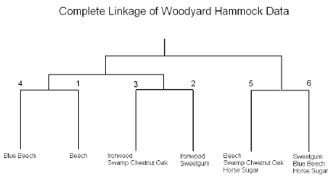
It is also useful to summarize the results in the cluster diagram:

We can see that the two ironwood clusters (2 and 3) are joined. Ironwood is an understory species that tend to be found in wet regions that may be frequently flooded. Cluster 2 also contains sweetgum, an overstory species found in disturbed habitats, while cluster 3 contains swamp chestnut oak, an overstory species characteristic of undisturbed habitats.
Clusters 5 and 6 both contain horse sugar, an understory species characteristic of light gaps in the forest. Cluster 5 also contains beech and swamp chestnut oak, two overstory species characteristic of undisturbed habitats. These are likely to be saplings of the two species growing in the horse sugar light gaps. Cluster 6 also contains blue beech, an understory species similar to ironwood, but characteristic of uplands.
Cluster 4 is dominated by blue beech, an understory species characteristic of uplands
Cluster 1 is dominated by beech, an overstory species most abundant in undisturbed habitats.
From the above description, you can see that a meaningful interpretation of the results of cluster analysis is best obtained using subject-matter knowledge.