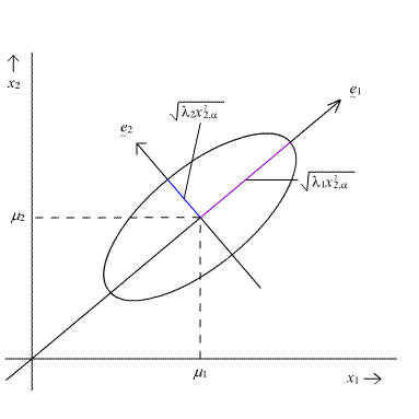
The geometry of the multivariate normal distribution can be investigated by considering the orientation, and shape of the prediction ellipse as depicted in the following diagram:

The \((1 - α) \times 100%\) prediction ellipse above is centered on the population means \(\mu_{1}\) and \(\mu_{2}\).
The ellipse has axes pointing in the directions of the eigenvectors \(e _ { 1 } , e _ { 2 } , \dots , e _ { p } \). Here, in this diagram for the bivariate normal, the longest axis of the ellipse points in the direction of the first eigenvector \(e_{1}\) and the shorter axis is perpendicular to the first, pointing in the direction of the second eigenvector \(e_{2}\).
The corresponding half-lengths of the axes are obtained by the following expression:
\(l_j = \sqrt{\lambda_j\chi^2_{p,\alpha}}\)
The plot above captures the lengths of these axes within the ellipse.
The volume (area) of the hyper-ellipse is equal to:
\(\dfrac{2\pi^{p/2}}{p\Gamma\left(\frac{p}{2}\right)}(\chi^2_{p,\alpha})^{p/2}|\Sigma|^{1/2}\)
In this expression for the volume (area) of the hyper-ellipse, \(Γ(x)\) is the gamma function. To compute the gamma function, consider the two special cases:
Case I: p is even
\(\Gamma\left(\frac{p}{2}\right) = \left(\frac{p}{2}-1\right)!\)
Case II: p is odd
\(\Gamma\left(\frac{p}{2}\right) = \dfrac{1 \times 3 \times 5 \times \dots \times (p-2) \times \sqrt{\pi}}{2^{(p-1)/2}}\)
We shall illustrate the shape of the multivariate normal distribution using the Wechsler Adult Intelligence Scale data.