4.2 - Bivariate Normal Distribution

Bivariate Normal Distribution Section

To further understand the multivariate normal distribution it is helpful to look at the bivariate normal distribution. Here our understanding is facilitated by being able to draw pictures of what this distribution looks like.

We have just two variables, \(X_{1}\) and \(X_{2}\), and these are bivariately normally distributed with mean vector components \(\mu_{1}\) and \(\mu_{2}\) and variance-covariance matrix shown below:

\(\left(\begin{array}{c}X_1\\X_2 \end{array}\right) \sim N \left[\left(\begin{array}{c}\mu_1\\ \mu_2 \end{array}\right), \left(\begin{array}{cc}\sigma^2_1 & \rho \sigma_1\sigma_2 \\ \rho\sigma_1\sigma_2 & \sigma^2_2 \end{array}\right)\right]\)

In this case, we have the variances for the two variables on the diagonal and on the off-diagonal, we have the covariance between the two variables. This covariance is equal to the correlation times the product of the two standard deviations. The determinant of the variance-covariance matrix is simply equal to the product of the variances times 1 minus the squared correlation.

\(|\Sigma| = \sigma^2_1\sigma^2_2(1-\rho^2)\)

The inverse of the variance-covariance matrix takes the form below:

\(\Sigma^{-1} = \dfrac{1}{\sigma^2_1\sigma^2_2(1-\rho^2)} \left(\begin{array}{cc}\sigma^2_2 & -\rho \sigma_1\sigma_2 \\ -\rho\sigma_1\sigma_2 & \sigma^2_1 \end{array}\right)\)

Joint Probability Density Function for Bivariate Normal Distribution: Substituting in the expressions for the determinant and the inverse of the variance-covariance matrix we obtain, after some simplification, the joint probability density function of (\(X_{1}\), \(X_{2}\)) for the bivariate normal distribution as shown below:; \(\phi(x_1,x_2) = \dfrac{1}{2\pi\sigma_1\sigma_2\sqrt{1-\rho^2}}\exp\{-\dfrac{1}{2(1-\rho^2)}\left[\left(\dfrac{x_1-\mu_1}{\sigma_1}\right)^2-2\rho \left(\dfrac{x_1-\mu_1}{\sigma_1}\right) \left(\dfrac{x_2-\mu_2}{\sigma_2}\right) + \left(\dfrac{x_2-\mu_2}{\sigma_2}\right)^2 \right]\}\)

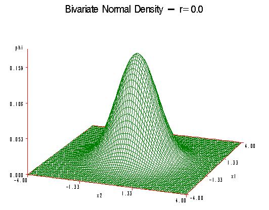
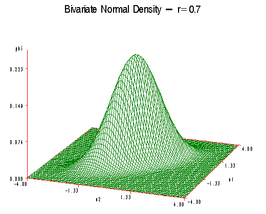
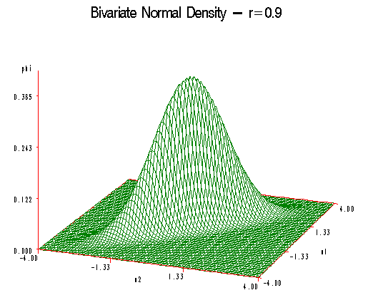
The following three plots are plots of the bivariate distribution for the various values for the correlation row.

The first plot shows the case where the correlation \(\rho\) is equal to zero. This special case is called the circular normal distribution. Here, we have a perfectly symmetric bell-shaped curve in three dimensions.

As ρ increases that bell-shaped curve becomes flattened on the 45-degree line. So for \(\rho\) equals 0.7 we can see that the curve extends out towards minus 4 and plus 4 and becomes flattened in the perpendicular direction.

Increasing \(\rho\) to 0.9 the curve becomes broader and the 45-degree line and even flatter still in the perpendicular direction.

These three curves were produced using the SAS program shown below. The desired correlation is specified in the third line of the SAS code (here at 0.9). No other changes are required to run this program. It would be a good idea to try this program for various values of r between -1 and 1 to explore how the shape of the normal distribution varies with the correlation.

Note: In the upper right-hand corner of the code block you will have the option of copying () the code to your clipboard or downloading () the file to your computer.

options ls=78;   /*This sets the max number of lines per page to 78.*/
title "Bivariate Normal Density";   /*This sets a title that will appear on each page of the output until it's changed.*/
%let r=0.9;   /*This defines the macro variable r; it will be referenced with &r throughout the code.*/
data a;   /*This data set defines the coordinates for plotting the bivariate normal pdf. The domain is the square of values between -4 and 4 for both x1 and x2. And phi represents the value of the normal pdf as a function of both x1 and x2.*/
  pi=3.1416;   
  do x1=-4 to 4 by 0.1;   
    do x2=-4 to 4 by 0.1;   
      phi=exp(-(x1*x1-2*&r*x1*x2+x2*x2)/2/(1-&r*&r))/2/pi/sqrt(1-&r*&r);   
      output;   
    end;   
  end;   
  run;   
proc g3d;   /*This plots in 3d the bivariate pdf for the variables x1, x2, and phi defined in the data set "a" above. The viewing angle is determined by the 'rotate' option.*/
  plot x1*x2=phi / rotate=-20;   
  run;

Note! This code assumes that the variances are both equal to one.

How to Use Minitab to Create Plots of the Bivariate Distribution.

You will need the formula that is found in the downloadable text file here: phi_equation_r=0.7.txt.

4.2 - Bivariate Normal Distribution

Bivariate Normal Distribution Section

Using Technology Section

How to Use Minitab to Create Plots of the Bivariate Distribution.

To plot a bivariate normal density for a given correlation value: