To test for treatment by time interactions we need to carry out a Profile Analysis. We can create a Profile Plot as shown in the Dog SAS program. (This program is similar in structure to swiss13a.sas used in Hotelling's T-square lesson previously.)
Here, we want to plot the treatment means against time for each of our four treatments. We can then examine the form the interactions take if they are deemed significant.
Note: In the upper right-hand corner of the code block you will have the option of copying ( ) the code to your clipboard or downloading ( ) the file to your computer.
options ls=78;
title "Profile Plot - Dog Data";

 /* After reading in the dog1 data, the variables are stacked
  * into two columns, one named 'time' for the time points and
  * one named 'k' for the quantitative response values.
  * The original p1 through p4 responses are removed.
  */

data dogs;
  infile "D:\Statistics\STAT 505\data\dog1.csv" firstobs=2 delimiter=',';
  input treat dog p1 p2 p3 p4;
  time=1;  k=p1; output;
  time=5;  k=p2; output;
  time=9;  k=p3; output;
  time=13; k=p4; output;
  drop p1 p2 p3 p4;
  run;

 /* This sorts the data by both treat and time.
  * The priority is to sort by treat first, then time
  */

proc sort data=dogs;
  by treat time;
  run;

 /* This calculates the mean response k for each level
  * of treat and time. The results are saved in a separate
  * file called 'a' with means stored as 'mean'.
  */

proc means data=dogs;
  by treat time;
  var k;
  output out=a mean=mean;

filename t1 "dog.ps";
goptions device=ps300 gsfname=t1 gsfmode=replace;

 /* The axis commands define the size of the plotting window.
  * The plot statement specifies the mean for each time and treat
  * are to be plotted but with separate lines for treat.
  * Each treat group is given a different symbol for distinction.
  * /

proc gplot;
  axis1 length=4 in;
  axis2 length=6 in;
  plot mean*time=treat / vaxis=axis1 haxis=axis2;
  symbol1 v=J f=special h=2 i=join color=black;
  symbol2 v=K f=special h=2 i=join color=black;
  symbol3 v=L f=special h=2 i=join color=black;
  symbol4 v=M f=special h=2 i=join color=black;
  run;
Repeated measures profile plot
To create a profile plot for the repeated measures model:
- Open the ‘dog1’ data set in a new worksheet
- Rename the columns treat, dog, p1, p2, p3, and p4, from left to right.
- Graph > Line plot > Multiple Y’s
- Highlight and select p1 through p4 to move these to the Graph window.
- Highlight and select treat to move this to the Categorical variable window.
- Choose 'OK'. The profile plot is shown in the results area.
This program plots the treatment means against time, separately for each treatment. Here, the means for treatment 1 are given by the circles, treatment 2 squares, treatment 3 triangles, and treatment 4 stars.
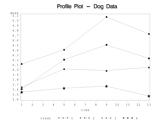
The test for interaction tests the hypothesis that these line segments are parallel to one another.
To test for interaction, we define a new data vector for each observation. Here we consider the data vector for dog j receiving treatment i. This data vector is obtained by subtracting the data from time 2 minus the data from time 1, the data from time 3 minus the data from time 2, and so on...
This yields the vector of differences between successive times and is expressed as follows:
\(\mathbf{Z}_{ij} = \left(\begin{array}{c}Z_{ij1}\\ Z_{ij2} \\ \vdots \\ Z_{ij, t-1}\end{array}\right) = \left(\begin{array}{c}Y_{ij2}-Y_{ij1}\\ Y_{ij3}-Y_{ij2} \\ \vdots \\Y_{ijt}-Y_{ij,t-1}\end{array}\right)\)
Because this vector is a function of the random data, it is a random vector, and so has a population mean. Thus, for treatment i, we define the population mean vector \(E(\mathbf{Z}_{ij}) = \boldsymbol{\mu}_{Z_i}\).
Then we will perform a MANOVA on these \(Z_{ij}\)'s to test the null hypothesis that
\(H_0\colon \boldsymbol{\mu}_{Z_1} = \boldsymbol{\mu}_{Z_2} = \dots = \boldsymbol{\mu}_{Z_a} \)
The SAS program carries out this MANOVA procedure in the third MANOVA statement as highlighted below:
Note: In the upper right-hand corner of the code block you will have the option of copying ( ) the code to your clipboard or downloading ( ) the file to your computer.
options ls=78;
title "Repeated Measures - Coronary Sinus Potassium in Dogs";


data dogs;
  infile "D:\Statistics\STAT 505\data\dog1.csv" firstobs=2 delimiter=',';
  input treat dog p1 p2 p3 p4;
  run;

proc print data=dogs;
  run;

 /* The class statement specifies treat as a categorical variable.
  * The model statement specifies p1 through p4 as the responses
  * and treat as the factor.
  * The h= option in the manova statement is used to specify over
  * which groups the mean response vectors are to be compared.
  * The m= option specifies the transformation (if any) to be
  * applied to the responses before the means are calculated.
  */

proc glm data=dogs;
  class treat;
  model p1 p2 p3 p4=treat;
  manova h=treat / printe;
  manova h=treat m=p1+p2+p3+p4;
  manova h=treat m=p2-p1,p3-p2,p4-p3;
  run;
To fit the MANOVA model and test for interaction effect
- Open the ‘dog1’ data set in a new worksheet
- Rename the columns treat, dog, p1, p2, p3, and p4, from left to right.
- Name new columns in the worksheet diff12, diff23, diff34. These will be used below.
- Calc > Calculator
- Highlight and select diff12 for the Store result window.
- In the Expression window, enter p1-p2, and choose OK. The first difference of the responses appears in the diff12 column in the worksheet.
- Repeat steps a. and b. but with diff23 in the Store result window and with p2-p3 in the Expression window.
- Repeat steps a. and b. but with diff34 in the Store result window and with p3-p4 in the Expression window.
- Stat > ANOVA > General MANOVA
- Highlight and select diff12, diff23, and diff34 to move these to the Responses window.
- Highlight and select treat to move it to the Model window.
- Choose OK. The results for the interaction test are displayed in the results area.
In the third MANOVA statement, we are testing for interaction between treatment and time. We obtain the vector Z, by setting m equal to the differences between the data at different times. i.e., p2-p1, p3-p2, and p4-p3. This will carry out the profile analysis, or equivalently, test for interactions between treatment and time.
Let's look at the output. Again, be careful when you look at the results to make sure you are in the right part of the output.
| p1 | p2 | p3 | p4 | |
|---|---|---|---|---|
| MVAR1 | -1 | 1 | 0 | 0 |
| MVAR2 | 0 | -1 | 1 | 0 |
| MVAR3 | 0 | 0 | -1 | 1 |
Find the table with the kind of function used in defining the vector MVAR, comprised of the elements MVAR1, MVAR2, and MVAR3.
For MVAR1 we have minus p1 plus p2, for MVAR 2 we have minus p2 plus p3, and so on...
The results are then found below this table in the SAS output:
| Statistic | Value | F Value | Num DF | Den DF | Pr > F |
|---|---|---|---|---|---|
| Wilks' Lambda | 0.59835958 | 1.91 | 9 | 73.163 | 0.0637 |
| Pillai's Trace | 0.44352640 | 1.85 | 9 | 96 | 0.0689 |
| Hotelling-Lawley Trace | 0.60246548 | 1.96 | 9 | 44.068 | 0.0672 |
| Roy's Greatest Root | 0.46206108 | 4.93 | 3 | 32 | 0.0063 |
NOTE: F Statistic for Roy's Greatest Root is an upper bound.
Here we get a Wilks Lambda of 0.598 with a supporting F-value of 1.91 with 9 and 73 d.f.
This p-value is not significant if we strictly adhere to the 0.05 significance level.
Conclusion Section
There is weak evidence that the effect of treatment depends on time \( \left( \Lambda = 0.598; F = 1.91; d. f. = 9, 73; p = 0.0637 \right) \).
By reporting the p-value with our results, we allow the reader to make their own judgment regarding the significance of the test. Conservative readers might say that 0.0637 is not significant and categorically state that this is not significant, inferring that there is no evidence for an interaction. More liberal readers, however, might say that this is very close and consider this weak evidence for an interaction. When you report the results in this form, including the p-value, you allow the reader to make their own judgment.