The following shows two examples to construct orthogonal contrasts. In each example, we consider balanced data; that is, there are equal numbers of observations in each group.
Example 8-6: Section
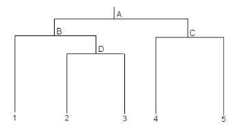
In some cases, it is possible to draw a tree diagram illustrating the hypothesized relationships among the treatments. In the following tree, we wish to compare 5 different populations of subjects. Prior to collecting the data, we may have reason to believe that populations 2 and 3 are most closely related. Populations 4 and 5 are also closely related, but not as close as populations 2 and 3. Population 1 is closer to populations 2 and 3 than populations 4 and 5.

Each branch (denoted by the letters A, B, C, and D) corresponds to a hypothesis we may wish to test. This yields the contrast coefficients as shown in each row of the following table:
| Contrasts | 1 | 2 | 3 | 4 | 5 |
|---|---|---|---|---|---|
| A | \(\dfrac{1}{3}\) | \(\dfrac{1}{3}\) | \(\dfrac{1}{3}\) | \(- \dfrac { 1 } { 2 }\) | \(- \dfrac { 1 } { 2 }\) |
| B | 1 | \(- \dfrac { 1 } { 2 }\) | \(- \dfrac { 1 } { 2 }\) | 0 | 0 |
| C | 0 | 0 | 0 | 1 | -1 |
| D | 0 | 1 | -1 | 0 | 0 |
Consider Contrast A. Here, we are comparing the mean of all subjects in populations 1,2, and 3 to the mean of all subjects in populations 4 and 5.
For Contrast B, we compare population 1 (receiving a coefficient of +1) with the mean of populations 2 and 3 (each receiving a coefficient of -1/2). Multiplying the corresponding coefficients of contrasts A and B, we obtain:
(1/3) × 1 + (1/3) × (-1/2) + (1/3) × (-1/2) + (-1/2) × 0 + (-1/2) × 0 = 1/3 - 1/6 - 1/6 + 0 + 0 = 0
So contrasts A and B are orthogonal. Similar computations can be carried out to confirm that all remaining pairs of contrasts are orthogonal to one another.
Example 8-7: Section
Consider the factorial arrangement of drug type and drug dose treatments:
| Drug | Low | High |
|---|---|---|
| A | 1 | 2 |
| B | 3 | 4 |
Here, treatment 1 is equivalent to a low dose of drug A, treatment 2 is equivalent to a high dose of drug A, etc. For this factorial arrangement of drug type and drug dose treatments, we can form the orthogonal contrasts:
| Contrasts | A, Low | A, High | B, Low | B, High |
|---|---|---|---|---|
| Drug | \(- \dfrac{1}{2}\) | \(- \dfrac{1}{2}\) | \( \dfrac{1}{2}\) | \( \dfrac{1}{2}\) |
| Dose | \(- \dfrac{1}{2}\) | \( \dfrac{1}{2}\) | \(- \dfrac { 1 } { 2 }\) | \( \dfrac{1}{2}\) |
| Interaction | \( \dfrac{1}{2}\) | \(- \dfrac{1}{2}\) | \(- \dfrac{1}{2}\) | \( \dfrac{1}{2}\) |
To test for the effects of drug type, we give coefficients with a negative sign for drug A, and positive signs for drug B. Because there are two doses within each drug type, the coefficients take values of plus or minus 1/2.
Similarly, to test for the effects of drug dose, we give coefficients with negative signs for the low dose, and positive signs for the high dose. Because there are two drugs for each dose, the coefficients take values of plus or minus 1/2.
The final test considers the null hypothesis that the effect of the drug does not depend on the dose, or conversely, the effect of the dose does not depend on the drug. In either case, we are testing the null hypothesis that there is no interaction between the drug and dose. The coefficients for this interaction are obtained by multiplying the signs of the coefficients for drug and dose. Thus, for drug A at the low dose, we multiply "-" (for the drug effect) times "-" (for the dose-effect) to obtain "+" (for the interaction). Similarly, for drug A at the high dose, we multiply "-" (for the drug effect) times "+" (for the dose-effect) to obtain "-" (for the interaction). The remaining coefficients are obtained similarly.
Example 8-8: Pottery Data Section
Recall the specific questions:
- Does the mean chemical content of pottery from Ashley Rails and Isle Thorns equal that of pottery from Caldicot and Llanedyrn?
- Does the mean chemical content of pottery from Ashley Rails equal that of pottery from Isle Thorns?
- Does the mean chemical content of pottery from Caldicot equal that of pottery from Llanedyrn?
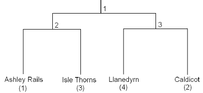
These questions correspond to the following theoretical relationships among the sites:

The relationships among sites suggested in the above figure suggest the following contrasts:
| Contrasts | Ashley Rails | Caldicot | Isle Thorns | Llanedyrn |
|---|---|---|---|---|
| 1 | \( \dfrac{1}{2}\) | \(- \dfrac{1}{2}\) | \( \dfrac{1}{2}\) | \(- \dfrac{1}{2}\) |
| 2 | 1 | 0 | -1 | 0 |
| 3 | 0 | 1 | 0 | -1 |
| \(n_i\) | 5 | 2 | 5 | 14 |
Notes
Contrasts 1 and 2 are orthogonal:
\[\sum_{i=1}^{g} \frac{c_id_i}{n_i} = \frac{0.5 \times 1}{5} + \frac{(-0.5)\times 0}{2}+\frac{0.5 \times (-1)}{5} +\frac{(-0.5)\times 0}{14} = 0\]
However, contrasts 1 and 3 are not orthogonal:
\[\sum_{i=1}^{g} \frac{c_id_i}{n_i} = \frac{0.5 \times 0}{5} + \frac{(-0.5)\times 1}{2}+\frac{0.5 \times 0}{5} +\frac{(-0.5)\times (-1) }{14} = \frac{6}{28}\]
Solution: Instead of estimating the mean of pottery collected from Caldicot and Llanedyrn by
\[\frac{\mathbf{\bar{y}_2+\bar{y}_4}}{2}\]
we can weigh by sample size:
\[\frac{n_2\mathbf{\bar{y}_2}+n_4\mathbf{\bar{y}_4}}{n_2+n_4} = \frac{2\mathbf{\bar{y}}_2+14\bar{\mathbf{y}}_4}{16}\]
Similarly, the mean of pottery collected from Ashley Rails and Isle Thorns may be estimated by
\[\frac{n_1\mathbf{\bar{y}_1}+n_3\mathbf{\bar{y}_3}}{n_1+n_3} = \frac{5\mathbf{\bar{y}}_1+5\bar{\mathbf{y}}_3}{10} = \frac{8\mathbf{\bar{y}}_1+8\bar{\mathbf{y}}_3}{16}\]
This yields the Orthogonal Contrast Coefficients:
| Contrasts | Ashley Rails | Caldicot | Isle Thorns | Llanedyrn |
|---|---|---|---|---|
| 1 | \( \dfrac{8}{16}\) | \(- \dfrac{2}{16}\) | \( \dfrac{8}{16}\) | \(- \dfrac{14}{16}\) |
| 2 | 1 | 0 | -1 | 0 |
| 3 | 0 | 1 | 0 | -1 |
| \(n_i\) | 5 | 2 | 5 | 14 |
The inspect button below will walk through how these contrasts are implemented in the SAS program.
Download the SAS program here: pottery.sas
Note: In the upper right-hand corner of the code block you will have the option of copying ( ) the code to your clipboard or downloading ( ) the file to your computer.
options ls=78;
title "MANOVA - Pottery Data";

data pottery;
  infile "D:\Statistics\STAT 505\data\pottery.csv" delimiter=',' firstobs=2;
  input site $ al fe mg ca na;
  run;

proc print data=pottery;
  run;

 /* The class statement specifies the categorical variable site.
  * The model statement specifies the five responses to the left
  * and the categorical predictor to the right of the = sign.
  */

proc glm data=pottery;
  class site;
  model al fe mg ca na = site;

 /* The contrast statements are used to calculate test statistics
  * and p-values for combinations of the groups.
  * The initial strings in quotes are arbitrary names,
  * followed by the name of the categorical variable defining the
  * groups, and the coefficients multiplying each group mean.
  */

  contrast 'C+L-A-I' site  8 -2  8 -14;
  contrast 'A vs I ' site  1  0 -1   0;
  contrast 'C vs L ' site  0  1  0  -1;

 /* The estimate statements are used to calculate estimates and
  * standard errors for combinations of the groups.
  * The divisor option divides the contrast by the value specified.
  */

  estimate 'C+L-A-I' site  8 -2  8 -14/ divisor=16;
  estimate 'A vs I ' site  1  0 -1   0;
  estimate 'C vs L ' site  0  1  0  -1;

 /* The lsmeans option provides standard error estimates and
  * standard errors for the differences between the site groups.
  * The manova statement is used for multivariate tests and results.
  * The h= option specifies the groups for comparison, and the
  * options printe and printh display the sums of squares and cross
  * products matrices for error and the hypothesis, respectively.
  */

  lsmeans site / stderr;
  manova h=site / printe printh;
  run;
Orthogonal contrast for MANOVA is not available in Minitab at this time.
Analysis
The following table of estimated contrasts is obtained
| Element | \(\widehat { \Psi } _ { 1 }\) | \(\widehat { \Psi } _ { 2 }\) | \(\widehat { \Psi } _ { 3 }\) |
|---|---|---|---|
| Al | 5.29 | -0.86 | -0.86 |
| Fe | -4.64 | -0.20 | -0.96 |
| Mg | -4.06 | -0.07 | -0.97 |
| Ca | -0.17 | 0.03 | 0.09 |
| Na | -0.17 | -0.01 | -0.20 |
These results suggest:
- Pottery from Ashley Rails and Isle Thorns have higher aluminum and lower iron, magnesium, calcium, and sodium concentrations than pottery from Caldicot and Llanedyrn.
- Pottery from Ashley Rails has higher calcium and lower aluminum, iron, magnesium, and sodium concentrations than pottery from Isle Thorns.
- Pottery from Caldicot has higher calcium and lower aluminum, iron, magnesium, and sodium concentrations than pottery from Llanedyrn.