Example 8-3: Pottery Data (MANOVA) Section
After we have assessed the assumptions, our next step is to proceed with the MANOVA.
This may be carried out using the Pottery SAS Program below.
Download the SAS Program here: pottery.sas
Note: In the upper right-hand corner of the code block you will have the option of copying ( ) the code to your clipboard or downloading ( ) the file to your computer.
options ls=78;
title "MANOVA - Pottery Data";

data pottery;
  infile "D:\Statistics\STAT 505\data\pottery.csv" delimiter=',' firstobs=2;
  input site $ al fe mg ca na;
  run;

proc print data=pottery;
  run;

 /* The class statement specifies the categorical variable site.
  * The model statement specifies the five responses to the left
  * and the categorical predictor to the right of the = sign.
  */

proc glm data=pottery;
  class site;
  model al fe mg ca na = site;

 /* The contrast statements are used to calculate test statistics
  * and p-values for combinations of the groups.
  * The initial strings in quotes are arbitrary names,
  * followed by the name of the categorical variable defining the
  * groups, and the coefficients multiplying each group mean.
  */

  contrast 'C+L-A-I' site  8 -2  8 -14;
  contrast 'A vs I ' site  1  0 -1   0;
  contrast 'C vs L ' site  0  1  0  -1;

 /* The estimate statements are used to calculate estimates and
  * standard errors for combinations of the groups.
  * The divisor option divides the contrast by the value specified.
  */

  estimate 'C+L-A-I' site  8 -2  8 -14/ divisor=16;
  estimate 'A vs I ' site  1  0 -1   0;
  estimate 'C vs L ' site  0  1  0  -1;

 /* The lsmeans option provides standard error estimates and
  * standard errors for the differences between the site groups.
  * The manova statement is used for multivariate tests and results.
  * The h= option specifies the groups for comparison, and the
  * options printe and printh display the sums of squares and cross
  * products matrices for error and the hypothesis, respectively.
  */

  lsmeans site / stderr;
  manova h=site / printe printh;
  run;
Performing a MANOVA
To carry out the MANOVA test in Minitab:
- Open the ‘pottery’ data set in a new worksheet
- For convenience, rename the columns: site, al, fe, mg, ca, and na from left to right.
- Stat > ANOVA > General MANOVA
- Highlight and select all five variables (al through na) to move them to the Responses window
- Highlight and select 'site' to move it to the Model window. Choose 'OK'.
- Choose 'OK' again. The MANOVA table is displayed in the results area.
Analysis
The concentrations of the chemical elements depend on the site where the pottery sample was obtained \(\left( \Lambda ^ { \star } = 0.0123; F = 13.09; \mathrm { d } . \mathrm { f } = 15,50 ; p < 0.0001 \right)\). It was found, therefore, that there are differences in the concentrations of at least one element between at least one pair of sites.
Question: How do the chemical constituents differ among sites?
A profile plot may be used to explore how the chemical constituents differ among the four sites. In a profile plot, the group means are plotted on the Y-axis against the variable names on the X-axis, connecting the dots for all means within each group. A profile plot for the pottery data is obtained using the SAS program below
Download the SAS Program here: pottery1.sas
Note: In the upper right-hand corner of the code block you will have the option of copying ( ) the code to your clipboard or downloading ( ) the file to your computer.
options ls=78;
title "Profile Plot for Pottery Data";

 /* After reading in the pottery data, where each variable is
  * originally in its own column, the next statements stack the data
  * so that all variable names are in one column called 'chemical',
  * and all response values are in another column called 'amount'.
  * This format is used for the calculations that follow, as well
  * as for the profile plot.
  */

data pottery;
  infile "D:\Statistics\STAT 505\data\pottery.csv" delimiter=',' firstobs=2;
  input site $ al fe mg ca na;
  chemical="al"; amount=al; output;
  chemical="fe"; amount=fe; output;
  chemical="mg"; amount=mg; output;
  chemical="ca"; amount=ca; output;
  chemical="na"; amount=na; output;

proc sort data=pottery;
  by site chemical;
  run;

 /* The means procedure calculates and saves the mean amount,
  * for each site and chemical. It then saves these results
  * in a new data set 'a' for use in the steps below.
  * /

proc means data=pottery;
  by site chemical;
  var amount;
  output out=a mean=mean;
  run;

 /* The axis commands define the size of the plotting window.
  * The horizontal axis is of the chemicals, and the vertical
  * axis is used for the means. Using the =site syntax also
  * separates these plotted means by site.
  * /

proc gplot data=a;
  axis1 length=3 in;
  axis2 length=4.5 in;
  plot mean*chemical=site / vaxis=axis1 haxis=axis2;
  symbol1 v=J f=special h=2 l=1 i=join color=black;
  symbol2 v=K f=special h=2 l=1 i=join color=black;
  symbol3 v=L f=special h=2 l=1 i=join color=black;
  symbol4 v=M f=special h=2 l=1 i=join color=black;
  run;
MANOVA profile plot
To create a profile plot in Minitab:
- Open the ‘pottery’ data set in a new worksheet
- For convenience, rename the columns: site, al, fe, mg, ca, and na from left to right.
- Graph > Line plots > Multiple Y’s
- Highlight and select all five variables (al through na) to move them to Graph variables.
- Highlight and select 'site' to move it to the Categorical variable for grouping.
- Choose 'OK'. The profile plot is displayed in the results area. Note that the order of the variables on the plot corresponds to the original order in the data set.
Analysis
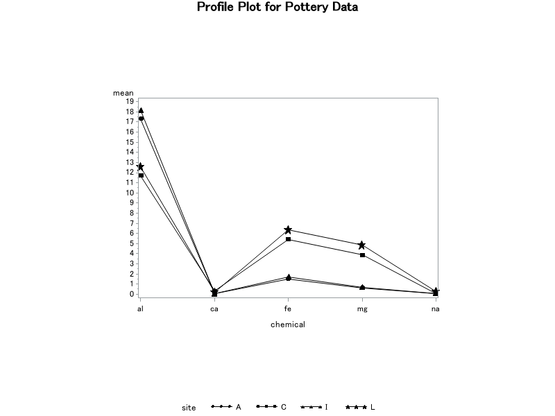
Results from the profile plots are summarized as follows:
- The sample sites appear to be paired: Ashley Rails with Isle Thorns and Caldicot with Llanedyrn.
- Ashley Rails and Isle Thorns appear to have higher aluminum concentrations than Caldicot and Llanedyrn.
- Caldicot and Llanedyrn appear to have higher iron and magnesium concentrations than Ashley Rails and Isle Thorns.
- Calcium and sodium concentrations do not appear to vary much among the sites.
Note: These results are not backed up by appropriate hypotheses tests. Hypotheses need to be formed to answer specific questions about the data. These should be considered only if significant differences among group mean vectors are detected in the MANOVA.
Specific Questions
- Which chemical elements vary significantly across sites?
- How do the sites differ?
- Is the mean chemical constituency of pottery from Ashley Rails and Isle Thorns different from that of Llanedyrn and Caldicot?
- Is the mean chemical constituency of pottery from Ashley Rails equal to that of Isle Thorns?
- Is the mean chemical constituency of pottery from Llanedyrn equal to that of Caldicot?
Analysis of Individual Chemical Elements
A naive approach to assessing the significance of individual variables (chemical elements) would be to carry out individual ANOVAs to test:
\(H_0\colon \mu_{1k} = \mu_{2k} = \dots = \mu_{gk}\)
for chemical k. Reject \(H_0 \) at level \(\alpha\) if
\(F > F_{g-1, N-g, \alpha}\)
Problem: If we're going to repeat this analysis for each of the p variables, this does not control for the experiment-wise error rate.
Just as we can apply a Bonferroni correction to obtain confidence intervals, we can also apply a Bonferroni correction to assess the effects of group membership on the population means of the individual variables.
Bonferroni Correction: Reject \(H_0 \) at level \(\alpha\) if
\(F > F_{g-1, N-g, \alpha/p}\)
or, equivalently, if the p-value is less than \(α/p\).
Example 8-4: Pottery Data (ANOVA) Section
The results for individual ANOVA results are output with the SAS program below.
Download the SAS program here: pottery.sas
Note: In the upper right-hand corner of the code block you will have the option of copying ( ) the code to your clipboard or downloading ( ) the file to your computer.
options ls=78;
title "MANOVA - Pottery Data";

data pottery;
  infile "D:\Statistics\STAT 505\data\pottery.csv" delimiter=',' firstobs=2;
  input site $ al fe mg ca na;
  run;

proc print data=pottery;
  run;

 /* The class statement specifies the categorical variable site.
  * The model statement specifies the five responses to the left
  * and the categorical predictor to the right of the = sign.
  */

proc glm data=pottery;
  class site;
  model al fe mg ca na = site;

 /* The contrast statements are used to calculate test statistics
  * and p-values for combinations of the groups.
  * The initial strings in quotes are arbitrary names,
  * followed by the name of the categorical variable defining the
  * groups, and the coefficients multiplying each group mean.
  */

  contrast 'C+L-A-I' site  8 -2  8 -14;
  contrast 'A vs I ' site  1  0 -1   0;
  contrast 'C vs L ' site  0  1  0  -1;

 /* The estimate statements are used to calculate estimates and
  * standard errors for combinations of the groups.
  * The divisor option divides the contrast by the value specified.
  */

  estimate 'C+L-A-I' site  8 -2  8 -14/ divisor=16;
  estimate 'A vs I ' site  1  0 -1   0;
  estimate 'C vs L ' site  0  1  0  -1;

 /* The lsmeans option provides standard error estimates and
  * standard errors for the differences between the site groups.
  * The manova statement is used for multivariate tests and results.
  * The h= option specifies the groups for comparison, and the
  * options printe and printh display the sums of squares and cross
  * products matrices for error and the hypothesis, respectively.
  */

  lsmeans site / stderr;
  manova h=site / printe printh;
  run;
MANOVA follow-up ANOVAs
To carry out multiple ANOVA tests in Minitab:
- Open the ‘pottery’ data set in a new worksheet
- For convenience, rename the columns: site, al, fe, mg, ca, and na from left to right.
- Stat > ANOVA > General Linear Model > Fit General Linear Model
- Highlight and select all five variables (al through na) to move them to the Responses window
- Highlight and select 'site' to move it to the Factors window.
- Choose 'OK'. Each of the ANOVA tables is displayed separately in the results area.
Analysis
Here, p = 5 variables, g = 4 groups, and a total of N = 26 observations. So, for an α = 0.05 level test, we reject
\(H_0\colon \mu_{1k} = \mu_{2k} = \dots = \mu_{gk}\)
if
\(F > F_{3,22,0.01} = 4.82\)
or equivalently, if the p-value reported by SAS is less than 0.05/5 = 0.01. The results of the individual ANOVAs are summarized in the following table. All tests are carried out with 3, 22 degrees freedom (the d.f. should always be noted when reporting these results).
| Element | F | SAS p-value |
|---|---|---|
| Al | 26.67 | < 0.0001 |
| Fe | 89.88 | < 0.0001 |
| Mg | 49.12 | < 0.0001 |
| Ca | 29.16 | < 0.0001 |
| Na | 9.50 | 0.0003 |
Because all of the F-statistics exceed the critical value of 4.82, or equivalently, because the SAS p-values all fall below 0.01, we can see that all tests are significant at the 0.05 level under the Bonferroni correction.
Conclusion: The means for all chemical elements differ significantly among the sites. For each element, the means for that element are different for at least one pair of sites.