Common Procedures in Minitab
Common Procedures in Minitab
Quick Links
Quick Links
Calculate a T-Interval for a Population Mean
Calculate a T-Interval for a Population MeanMinitab®
Procedure
A t-interval for a population mean provides an interval of estimates of the unknown population mean μ.
- Select Stat > Basic Statistics > 1 Sample t ...
- Use the pull-down options to select, 'Samples in columns.'
- Select the variable you want to analyze, (by double-clicking, or highlighting and clicking once on 'Select'.) so it appears in the box labeled 'Variables'.
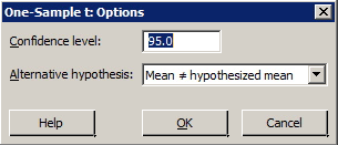
- Select 'Options' ... Type in the desired confidence level the default is 95.0 in the box labeled 'Confidence level'. (Ignore the box labeled 'Alternative'.)
- Select OK.
- Select OK. The output will appear in the session window.
Example
The US National Research Council currently recommends that females between the ages of 11 and 50 intake 15 milligrams of iron daily. The iron intakes of a random sample of 25 such American females are found in the dataset irondef.txt. With 95% confidence, what is the mean iron intake of all American females?
Minitab Dialog Boxes
Sample Minitab Output
One-Sample T: iron
| Variable | N | Mean | StDev | SE Mean | 95% CI |
|---|---|---|---|---|---|
| iron | 25 | 14.300 | 2.367 | 0.473 | (13.323, 15.277) |
Video Review
Code Numeric to Numeric Data
Code Numeric to Numeric DataMinitab®
Procedure
Minitab can be used to translate or "code" a column of numbers into another column of numbers. The procedure is particularly useful for creating dummy indicator variables for the qualitative predictor variables that you'd like to include in your regression model.
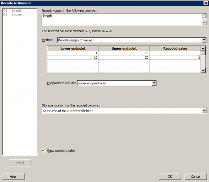
- In Minitab, select Data >> Recode >> to Numeric...
- In the box labeled Recode values in the following columns, specify the name of the numeric variable that you want to code.
- In the box labeled Method, specify a method for recoding the values specified above.
- For instance, to recode a range of values, type the numeric values in the boxes labeled Lower endpoint and Upper endpoint and the Recoded Value that you want this range to represent. Make sure you do this for every possible value of the variable that you want to code.
- Select OK. The new variable should appear in your worksheet.
Note: if you have more than one numeric variable to create, you have to code each one separately.
Example
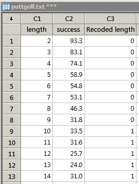
Sports Illustrated published results of a study designed to determine how well professional golfers putt. The data set puttgolf.txt contains data on the lengths of putts (x) and the percentage of successful putts (y) made by professional golfers during 15 tournaments. Only putts that were 2 to 20 feet from the hole are included in the data set. When fitting a two-piece piecewise linear regression function — connected at x = 10 — to the data, you have to create a new numeric dummy variable, say "dummy", that takes on value 0 if x ≤ 10 and 1 if x > 10. Use Minitab to code the numeric variable length into the numeric variable dummy.
Minitab Dialog Box
Resulting Minitab Worksheet
Video Review
Code a Text Variable into a Numeric Variable
Code a Text Variable into a Numeric VariableMinitab®
Procedure
Minitab can be used to translate or "code" a column of text values into another column of numeric values.
- In Minitab select Data >> Recode >> to Numeric...
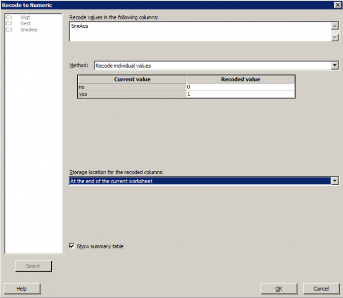
- In the box labeled Recode values in the following columns, specify the name of the text variable that you want to code.
- Under 'Method', select the option 'Recode individual values'.
- For each value of the variable that you want to code, type the text value in the box labeled Recoded value. Make sure you do this for every possible value of the text variable that you want to code.
- Select OK. The new numeric variable should appear in your worksheet. You can rename the column in your worksheet with a more effective label if you want.
Note: if you have more than one text variable to create, you have to code each one separately.
Example
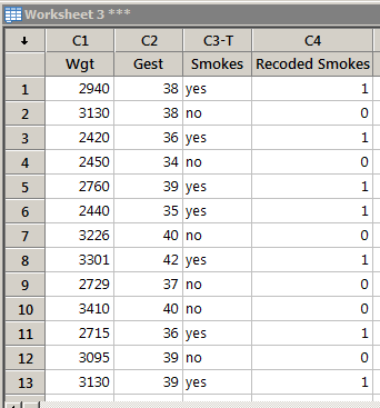
The data set birthsmokers2.txt contains data on the birthweight (y = Wgt), gestation length (x1 = Gest) and mother's smoking status (x2 = Smokes, yes or no) of babies born to 32 mothers. If you wanted to fit a multiple regression model that included smoking status, you'd first have to create a numeric variable in your worksheet, dummy say, that equals 1 if Smokes = yes and equals 0 if Smokes = no. Create the dummy variable in your worksheet.
Minitab Dialog Box
Resulting Minitab Worksheet
Video Review
Conduct Best Subsets Regression
Conduct Best Subsets RegressionMinitab® – Procedure
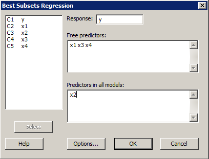
- Select Stat >> Regression >> Best Subsets...
- In the box labeled Response, specify the response.
- In the box labeled Free predictors, specify the predictors that you want considered for the model. (Do not include predictors that you specify in the following Predictors in all models box.)
- (Optional) In the box labeled Predictors in all models, specify all of the predictors that must be included in every model considered.
- Select OK. The output will appear in the session window.
Example
Researchers were interested in learning how the composition of cement affected the heat evolved during the hardening of the cement. Therefore, they measured and recorded the following data (cement.txt) on 13 batches of cement:
- Response y: heat evolved in calories during hardening of cement on a per gram basis
- Predictor x1: % of tricalcium aluminate
- Predictor x2: % of tricalcium silicate
- Predictor x3: % of tetracalcium alumino ferrite
- Predictor x4: % of dicalcium silicate
Perform a best subsets regression. In doing so, require that the predictor x2 be included in all models considered.
Minitab Dialog Box
Sample Output
Best Subsets Regression: y versus x1, x3, x4, x2
Response is y
The following variables are included in all models: x2
| Vars | R-Sq | Mallows | x | x | x | ||
|---|---|---|---|---|---|---|---|
| R-Sq(adj) | Cp | S | 1 | 3 | 4 | ||
| 1 | 97.9 | 97.4 | 2.7 | 2.4063 | x | ||
| 1 | 84.7 | 81.6 | 62.4 | 6.4455 | x | ||
| 2 | 98.2 | 97.6 | 3.0 | 2.3087 | x | x | |
| 2 | 98.2 | 97.6 | 3.0 | 2.3121 | x | x | |
| 3 | 98.2 | 97.4 | 5.0 | 2.4460 | x | x | x |
Video Review
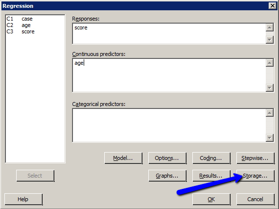
Conduct Regression Error Normality Tests
Conduct Regression Error Normality TestsMinitab® – Procedure
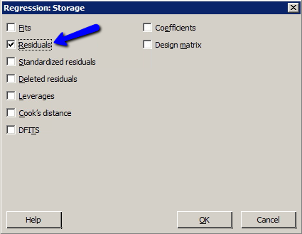
If you haven't already done so, store the residuals on which you want to conduct the Ryan Joiner correlation test.
- Select Stat > Regression > Regression > Fit Regression Model...
- Specify the response and the predictor variable(s).
- Select Storage... Under Diagnostic Measures, select the type of residuals (and/or influence measures) that you want to store. Select OK.
- Select OK. The requested residuals (and/or influence measures) will be stored in your worksheet.
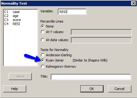
Once Minitab has stored the residuals in your worksheet:
- Select Stat > Basic Statistics > Normality Test...
- In the box labeled Variable, specify the name of the variable containing the residuals (Minitab names it something like RESI1, RESI2, ...).
- Under Tests for Normality, select Anderson-Darling, Ryan-Joiner, or Kolmogorov-Smirnov.
- Select OK. A new graph window containing the requested normal probability plot should appear.
Example
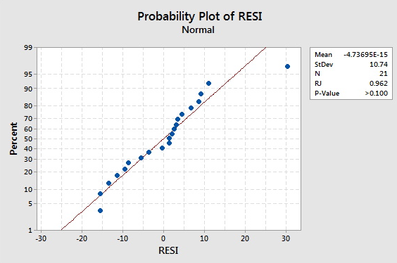
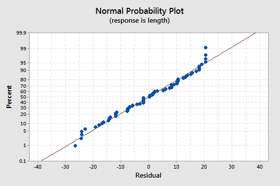
The data set adaptive.txt contains the Gesell adaptive scores and ages (in months) of n = 21 children with cyanotic heart disease. Upon regressing the response y = score on the predictor x = age, use the resulting residuals to test whether or not the error terms are normally distributed.
Minitab Dialog Boxes
Sample Output
Video Review
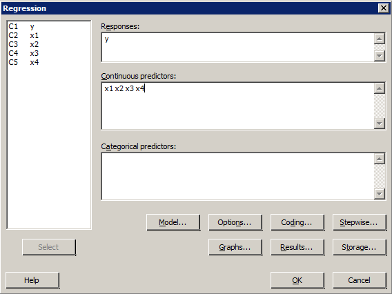
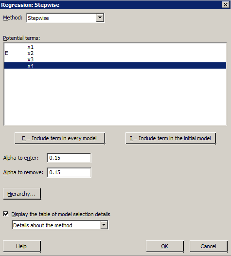
Conduct Stepwise Regression
Conduct Stepwise RegressionMinitab® – Procedure
- Select Stat >> Regression >> Regression >> Fit Regression Model...
- In the box labeled Response, specify the response.
- In the box labeled Continuous Predictors, specify all the predictors that you want to be considered for the model.
- Click on the Stepwise button.
- Choose 'Stepwise' from among the Method pull-down options.
- (Optional) Use the buttons below the box labeled Potential terms to indicate terms to include in every model, specify all of the predictors that must be included in every model considered.
- (Optional) Specify the Alpha to enter and Alpha to remove significance levels. The default for both is 0.15.
- Check the box labeled 'Display the table of model selection details using the pull-down to select 'Include details for each step'.
- Select OK.
- Select OK. The output will appear in the session window.
Example
Researchers were interested in learning how the composition of cement affected the heat evolved during the hardening of the cement. Therefore, they measured and recorded the following data (cement.txt) on 13 batches of cement:
- Response y: heat evolved in calories during hardening of cement on a per gram basis
- Predictor x1: % of tricalcium aluminate
- Predictor x2: % of tricalcium silicate
- Predictor x3: % of tetracalcium alumino ferrite
- Predictor x4: % of dicalcium silicate
Perform stepwise regression on the data set. Let αE = αR = 0.15. In doing so, require that the predictor x2 be included in all models considered.
Minitab Dialog Boxes
Sample Output
Regression analysis: y versus x1, x2, x3, x4
Stepwise Selection of Terms
Candidate terms: x1, x2, x3, x4
| Terms | --------Step 1-------- | --------Step 2-------- | ||
|---|---|---|---|---|
| Coef | P | Coef | P | |
| Constant | 57.42 | 52.58 | ||
| x2 | 0.789 | 0.001 | 0.6623 | 0.000 |
| x1 | 1.468 | 0.000 | ||
| S | 9.07713 | 2.40634 | ||
| R-sq | 66.63% | 97.87% | ||
| R-sq(adj) | 63.59% | 97.44% | ||
| R-sq(pred) | 55.74% | 96.54% | ||
| Mallows' Cp | 142.49 | 2.68 | ||
\(\alpha\) to enter = 0.15, \(\alpha\) to remove = 0.15 At your request, the stepwise procedure included these terms in every module: x2
Video Review
Conduct a Lack of Fit Test
Conduct a Lack of Fit TestMinitab®
Procedure
- Select Stat >> Regression >> Regression ... >> Fit Regression Model ...
- Specify the response and the predictor(s).
- Minitab automatically recognizes replicates of data and produces the Lack of Fit test with Pure error by default.
- Select OK. The output will appear in the session window.
Example
The data set bluegills.txt contains the lengths (in mm) and ages (in years) of n = 78 bluegill fish. Is there sufficient evidence to conclude that there is a lack of linear fit between y = length and x = age of bluegill fish?
Minitab Dialog Box

Sample Output
Regression Analysis: length versus age
| Analysis of Variance | |||||
|---|---|---|---|---|---|
| Source | DF | Adj SS | Adj MS | F-value | P-value |
| Regression | 1 | 32966 | 32965.8 | 210.66 | 0.000 |
| age | 1 | 32966 | 32965.8 | 210.66 | 0.000 |
| Error | 76 | 11893 | 156.5 | ||
|
Lack-of-Fit |
4 | 3080 |
770.0 |
6.29 | 0.000 |
| Pure Error | 72 | 8813 | 122.4 | ||
| Total | 77 | 44859 | |||
Video Review
Conducting a Hypothesis Test for the Population Correlation Coefficient P
Conducting a Hypothesis Test for the Population Correlation Coefficient PThere is one more point we haven't stressed yet in our discussion about the correlation coefficient r and the coefficient of determination r2 — namely, the two measures summarize the strength of a linear relationship in samples only. If we obtained a different sample, we would obtain different correlations, different r2 values, and therefore potentially different conclusions. As always, we want to draw conclusions about populations, not just samples. To do so, we either have to conduct a hypothesis test or calculate a confidence interval. In this section, we learn how to conduct a hypothesis test for the population correlation coefficient ρ (the Greek letter "rho").
Incidentally, where does this topic fit in among the four regression analysis steps?
- Model formulation
- Model estimation
- Model evaluation
- Model use
It's a situation in which we use the model to answer a specific research question, namely whether or not a linear relationship exists between two quantitative variables
In general, a researcher should use the hypothesis test for the population correlation ρ to learn of a linear association between two variables, when it isn't obvious which variable should be regarded as the response. Let's clarify this point with examples of two different research questions.
We previously learned that to evaluate whether or not a linear relationship exists between skin cancer mortality and latitude, we can perform either of the following tests:
- t-test for testing H0: β1= 0
- ANOVA F-test for testing H0: β1= 0
That's because it is fairly obvious that latitude should be treated as the predictor variable and skin cancer mortality as the response. Suppose we want to evaluate whether or not a linear relationship exists between a husband's age and his wife's age? In this case, one could treat the husband's age as the response:
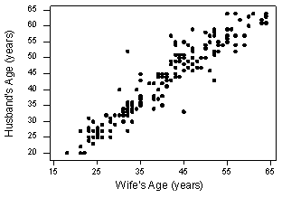
- Pearson correlation of HAge and WAge = 0.939
or one could treat wife's age as the response:
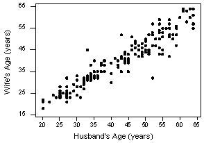
Pearson correlation of HAge and WAge = 0.939
In cases such as these, we answer our research question concerning the existence of a linear relationship by using the t-test for testing the population correlation coefficient H0: ρ = 0.
Let's jump right to it! We follow standard hypothesis test procedures in conducting a hypothesis test for the population correlation coefficient ρ. First, we specify the null and alternative hypotheses:
Null hypothesis H0: ρ = 0
Alternative hypothesis HA: ρ ≠ 0 or HA: ρ < 0 or HA: ρ > 0
Second, we calculate the value of the test statistic using the following formula:
Test statistic: \(t^*=\frac{r\sqrt{n-2}}{\sqrt{1-r^2}}\)
Third, we use the resulting test statistic to calculate the P-value. As always, the P-value is the answer to the question "how likely is it that we’d get a test statistic t* as extreme as we did if the null hypothesis were true?" The P-value is determined by referring to a t-distribution with n-2 degrees of freedom.
Finally, we make a decision:
- If the P-value is smaller than the significance level α, we reject the null hypothesis in favor of the alternative. We conclude "there is sufficient evidence at the α level to conclude that there is a linear relationship in the population between the predictor x and response y."
- If the P-value is larger than the significance level α, we fail to reject the null hypothesis. We conclude "there is not enough evidence at the α level to conclude that there is a linear relationship in the population between the predictor x and response y."
Let's perform the hypothesis test on the husband's age and wife's age data in which the sample correlation based on n = 170 couples is r = 0.939. To test H0: ρ = 0 against the alternative HA: ρ ≠ 0, we obtain the following test statistic:
\[t^*=\frac{r\sqrt{n-2}}{\sqrt{1-r^2}}=\frac{0.939\sqrt{170-2}}{\sqrt{1-0.939^2}}=35.39\]
To obtain the P-value, we need to compare the test statistic to a t-distribution with 168 degrees of freedom (since 170 - 2 = 168). In particular, we need to find the probability that we'd observe a test statistic more extreme than 35.39, and then, since we're conducting a two-sided test, multiply the probability by 2. Minitab helps us out here:
| Student's t distribution with 168 DF | |
|---|---|
| x | P ( X <= x ) |
| 35.3900 | 1.0000 |
The output tells us that the probability of getting a test statistic smaller than 35.39 is greater than 0.999. Therefore, the probability of getting a test statistic greater than 35.39 is less than 0.001. As illustrated in this ![]() , we multiply by 2 and determine that the P-value is less than 0.002. Since the P-value is small — smaller than 0.05, say — we can reject the null hypothesis. There is sufficient statistical evidence at the α = 0.05 level to conclude that there is a significant linear relationship between a husband's age and his wife's age.
, we multiply by 2 and determine that the P-value is less than 0.002. Since the P-value is small — smaller than 0.05, say — we can reject the null hypothesis. There is sufficient statistical evidence at the α = 0.05 level to conclude that there is a significant linear relationship between a husband's age and his wife's age.
Incidentally, we can let statistical software like Minitab do all of the dirty work for us. In doing so, Minitab reports:
| Pearson correlation of WAge and HAge= 0.939 | |
|---|---|
| P-Value = 0.000 |
It should be noted that the three hypothesis tests we learned for testing the existence of a linear relationship — the t-test for H0: β1= 0, the ANOVA F-test for H0: β1= 0, and the t-test for H0: ρ = 0 — will always yield the same results. For example, if we treat the husband's age ("HAge") as the response and the wife's age ("WAge") as the predictor, each test yields a P-value of 0.000... < 0.001:
| The regression equation is HAge= 3.59 + 0.967 WAge 170 cases used 48 cases contain missing values |
|||||
|---|---|---|---|---|---|
| Predictor | Coef | SE Coef | T | P | |
| Constant | 3.590 | 1.159 | 3.10 | 0.002 | |
| WAge | 0.96670 | 0.02742 | 35.25 | 0.000 | |
| S = 4.069 | R-Sq = 88.1% | R-sq(adj) = 88.0% | |||
| Analysis of Variance | |||||
| Source | DF | SS | MS | F | P |
| Regression | 1 | 20577 | 20577 | 1242.51 | 0.000 |
| Error | 168 | 2782 | 17 | ||
| Total | 169 | 23359 | |||
| Pearson correlation of WAge and HAge = 0.939 P-Value = 0.000 |
|||||
And similarly, if we treat the wife's age ("WAge") as the response and the husband's age ("HAge") as the predictor, each test yields of P-value of 0.000... < 0.001:
| The regression equation is WAge= 1.57 + 0.911 HAge 170 cases used 48 cases contain missing values |
|||||
|---|---|---|---|---|---|
| Predictor | Coef | SE Coef | T | P | |
| Constant | 1.574 | 1.150 | 1.37 | 0.173 | |
| WAge | 0.91124 | 0.02585 | 35.25 | 0.000 | |
| S = 3.951 | R-Sq = 88.1% | R-sq(adj) = 88.0% | |||
| Analysis of Variance | |||||
| Source | DF | SS | MS | F | P |
| Regression | 1 | 19396 | 19396 | 1242.51 | 0.000 |
| Error | 168 | 2623 | 17 | ||
| Total | 169 | 22019 | |||
| Pearson correlation of WAge and HAge = 0.939 P-Value = 0.000 |
|||||
Technically, then, it doesn't matter what test you use to obtain the P-value. You will always get the same P-value. But, you should report the results of the test that make sense for your particular situation:
- If one of the variables can be clearly identified as the response, report that you conducted a t-test or F-test results for testing H0: β1 = 0. (Does it make sense to use x to predict y?)
- If it is not obvious which variable is the response, report that you conducted a t-test for testing H0: ρ = 0. (Does it only make sense to look for an association between x and y?)
One final note ... as always, we should clarify when it is okay to use the t-test for testing H0: ρ = 0? The guidelines are a straightforward extension of the "LINE" assumptions made for the simple linear regression model. It's okay:
- When it is not obvious which variable is the response.
- When the (x, y) pairs are a random sample from a bivariate normal population.
- For each x, the y's are normal with equal variances.
- For each y, the x's are normal with equal variances.
- Either, y can be considered a linear function of x.
- Or, x can be considered a linear function of y.
- The (x, y) pairs are independent
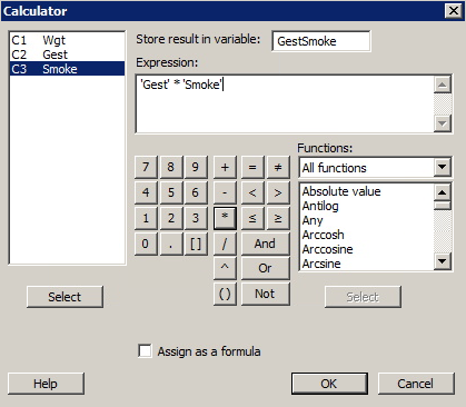
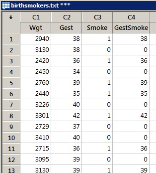
Create Interaction Variables
Create Interaction VariablesMinitab® – Procedure
In order to enter interaction terms into a regression model in Minitab, you have to first create column(s) in the worksheet that contains the interaction term(s).
- Select Calc >> Calculator...
- In the box labeled Store the result in variable, specify the column (or the name of the new variable, x1x2, for example) in which you want to store the interaction term.
- In the box labeled Expression, multiply the two predictor variables that go into the interaction terms. For example, if you want to create an interaction between x1 and x2, use the calculator to multiply them together: 'x1'*'x2'.
- Select OK. The new variable, x1x2, should appear in your worksheet.
Example
The data set birthsmokers.txt contains data on the birthweight (y = Wgt), gestation length (x1 = Gest) and (x2 = Smoke, 1 if mother smoked, 0 if not) of babies born to 32 mothers. If you wanted to fit a multiple regression model that allowed interaction between gestation length and smoking, you'd first have to create a variable in your worksheet, GestSmoke say, that contained the interaction term. Use Minitab's calculator to create the interaction term in your worksheet.
Minitab Dialog Box
Sample of Resulting Minitab Worksheet
Video Review
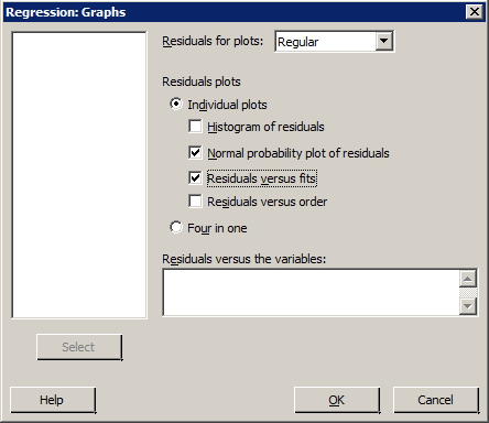
Create Residual Plots
Create Residual PlotsMinitab® – Procedure
- Select Stat >> Regression >> Regression ... >> Fit Regression Model ...
- Specify the response and the predictor(s).
- Under Graphs...
- Under Residuals for Plots, select either Regular or Standardized.
- Under Residuals Plots, select the desired types of residual plots. If you want to create residuals vs. predictor plot, specify the predictor variable in the box labeled Residuals versus the variables.
- Select OK.
- Select OK. The standard regression output will appear in the session window, and the residual plots will appear in new windows.
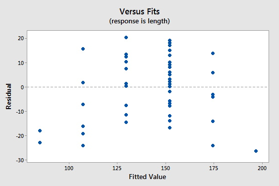
Example
The data set bluegills.txt contains the lengths (in mm) and ages (in years) of n = 78 bluegill fish. Treating y = length as the response and x = age as the predictor, request a normal plot of the standardized residuals and a standardized residuals vs. fits plot.
Minitab dialog boxes
Sample output
Video Review
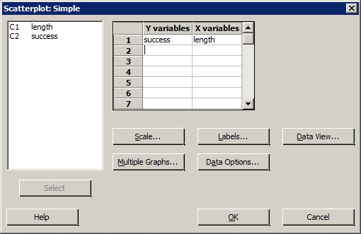
Create a Basic Scatter Plot
Create a Basic Scatter PlotMinitab® – Procedure
The basic "scatter plot" command creates a simple scatter plot of a response variable y against a predictor variable x.
- Select Graph >> Scatterplot ...
- Select the graph type "Simple."
- Specify your Y variable and your X variable in the boxes provided.
- Select OK. A new window containing the scatter plot will appear.
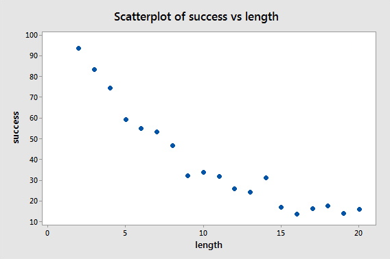
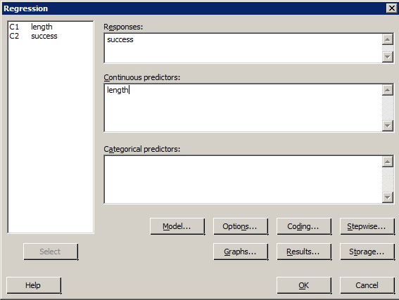
Example
Sports Illustrated published results of a study designed to determine how well professional golfers putt. The data set puttgolf.txt contains data on the lengths of putts and the percentage of successful putts made by professional golfers during 15 tournaments. Only putts that were 2 to 20 feet from the hole are included in the data set.
What do the plot of y = success and x = length suggest about the relationship between the two variables?
Minitab Dialog Box
Minitab Sample Plot
Video Review
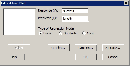
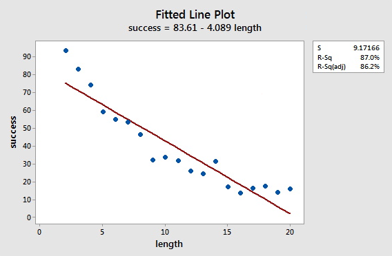
Create a Fitted Line Plot
Create a Fitted Line PlotMinitab® – Procedure
The "fitted line plot" command is one way of obtaining the estimated regression function between a response y and a predictor x. The "fitted line plot" command provides not only the estimated regression function but also a scatter plot of the data adorned with the estimated regression function.
- Select Stat >> Regression >> Fitted Line Plot...
- In the box labeled "Response (Y)", specify the desired response variable.
- In the box labeled "Predictor (X)", specify the desired predictor variable.
- Select OK. A new window containing the fitted line plot will appear.
Example
Sports Illustrated published results of a study designed to determine how well professional golfers putt. The data set puttgolf.txt contains data on the lengths of putts and the percentage of successful putts made by professional golfers during 15 tournaments. Only putts that were 2 to 20 feet from the hole are included in the data set.
What is the estimated linear relationship between y = success and x = length?
Minitab Dialog Box
Sample Output
Video Review
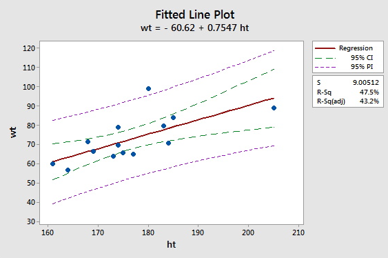
Create a Fitted Line Plot with Confidence and Prediction Bands
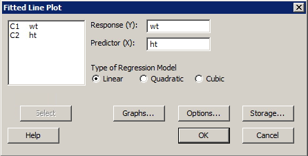
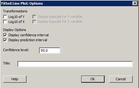
Create a Fitted Line Plot with Confidence and Prediction BandsMinitab® – Procedure
- Select Stat >> Regression >> Fitted line plot...
- Specify the response and the predictor.
- Select Options... Under Display Options, select Display confidence interval and select Display prediction interval. Specify the desired confidence level — 95% is the default. Select OK.
- Select OK. A new window containing the fitted line plot will appear.
Example
For people of the same age and gender, height is often considered a good predictor of weight. The data set htwtmales.txt contains the heights (ht, in cm) and weights (wt, in kg) of a sample of 14 males between the ages of 19 and 26 years.
- Find a 95% prediction band for the weight of a randomly selected male, aged 19 to 26.
- Find a 95% confidence band for the average weight of all males, aged 19 to 26.
Minitab Dialog Boxes
Sample Minitab Output Plot
Video Review
Create a Simple Matrix of Scatter Plots
Create a Simple Matrix of Scatter PlotsMinitab® – Procedure
Creating a matrix of scatter plots between a set of variables is a good way to visualize the relationship between each pair of variables.
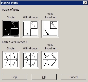
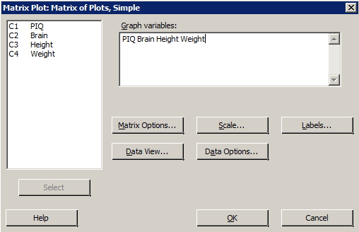
- Select Graph >> Matrix plot...
- Under Matrix of plots, select the Simple plot.
- In the box labeled Graph variables, specify the variables you want to include in your plot.
- Select OK. A new graph window should appear containing the scatter plot matrix.
Example
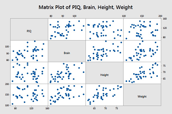
Using the dataset iqsize.txt, create a matrix of scatter plots between each pair of the four variables.
Minitab dialog boxes
Resulting scatter plot matrix
Video Review
Creating a Correlation Matrix
Creating a Correlation MatrixMinitab® – Procedure (v.16 & v.17)
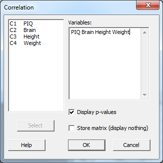
- Select Stat >> Basic statistics >> Correlation...
- In the box labeled Variables, specify the two (or more) variables for which you want the correlation coefficient(s) calculated.
- If you would like a P-value so that you can test that each population correlation is 0, put a checkmark in the box labeled Display p-values by clicking once on the box.
- Select OK. The output will appear in the session window.
Example
Using the iqsize.txt data set, estimate the correlations among each pair of the four variables.
Minitab Dialog Box
Resulting Minitab Output
Correlations: PIQ, Brain, Height, Weight
| PIQ | Brain | Height | |
|---|---|---|---|
| Brain | 0.378 | ||
| 0.019 | |||
| Height | -0.093 | 0.588 | |
| 0.578 | 0.000 | ||
| Weight | 0.003 | 0.513 | 0.700 |
| 0.988 | 0.001 | 0.000 | |
P-Value
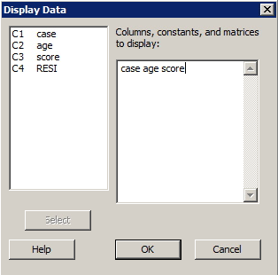
Display Data
Display DataMinitab® – Procedure
- In Minitab, select Data >> Display Data...
- In the box labeled Columns, constants, and matrices to display, specify the variables that you would like displayed.
- Select OK. The data will be displayed in the session window.
Example
Display the data contained in the adaptive.txt data set.
Minitab dialog box
Sample output
Results for: Worksheet 2
Data Display
| Row | case | age | score |
|---|---|---|---|
| 1 | 1 | 15 | 95 |
| 2 | 2 | 26 | 71 |
| 3 | 3 | 10 | 83 |
| 4 | 4 | 9 | 91 |
| 5 | 5 | 15 | 102 |
| 6 | 6 | 20 | 87 |
| 7 | 7 | 18 | 93 |
| 8 | 8 | 11 | 100 |
| 9 | 9 | 8 | 104 |
| 10 | 10 | 20 | 94 |
| 11 | 11 | 7 | 113 |
| 12 | 12 | 9 | 96 |
| 13 | 13 | 10 | 83 |
| 14 | 14 | 11 | 84 |
| 15 | 15 | 11 | 102 |
| 16 | 16 | 10 | 100 |
| 17 | 17 | 12 | 105 |
| 18 | 18 | 42 | 57 |
| 19 | 19 | 17 | 121 |
| 20 | 20 | 11 | 86 |
| 21 | 21 | 10 | 100 |
Video Review
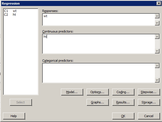
Find a Confidence Interval and a Prediction Interval for the Response
Find a Confidence Interval and a Prediction Interval for the ResponseMinitab® – Procedure
- Select Stat >> Regression >> Regression >> Fit Regression Model ...
- Specify the response and the predictor(s).
- Select OK. The output will appear in the session window.
Next, back up to the Main Menu having just run this regression:
- Select Stat >> Regression >> Regression >> Predict ...
- Specify the response.
- Specify either the x value ("Enter individual values") or a column name ("Enter columns of values") containing multiple x values.
- Select Options... Specify the Confidence level — the default is 95%. Select OK.
- Select OK. The output will appear in the session window.
Example
For people of the same age and gender, height is often considered a good predictor of weight. The data set htwtmales.txt contains the heights (ht, in cm) and weights (wt, in kg) of a sample of 14 males between the ages of 19 and 26 years.
- Find a 95% prediction interval for the weight of a randomly selected male, aged 19 to 26, who is 170 centimeters tall.
- Find a 95% confidence interval for the average weight of all males, aged 19 to 26, who are 170 centimeters tall.
Minitab Dialog Boxes
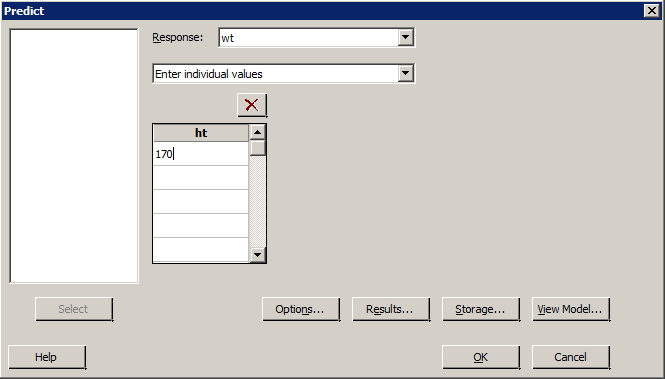
Resulting Sample Minitab Output
Prediction for wt
Regression Equation
wt = -60.6 + 0.755 ht
| Variable | Setting | no heading | no heading | ||
|---|---|---|---|---|---|
| ht | 170 | ||||
| Fit | SE Fit | 95% CI | 95%PI | ||
| 67.6694 | 2.83819 | (61.4855, 73.8533) | (47.0975, 88.2413) | ||
Video Review
Find a t Critical Value
Find a t Critical ValueMinitab® – Procedure
You may need to find a t critical value if you are using the critical value approach to conduct a hypothesis test that uses a t-statistic.
- Select Calc >> Probability Distributions >> t ...
- Click the button labeled 'Inverse cumulative probability'. (Ignore the box labeled 'Noncentrality parameter'. That is, leave the default value of 0 as is.)
- Type in the number of degrees of freedom in the box labeled 'Degrees of Freedom'.
- Click the button labeled 'Input Constant'. In the box, type the cumulative probability for which you want to find the associated t-value.
- Select OK. The t-value will appear in the session window.
Example
The US National Research Council currently recommends that females between the ages of 11 and 50 intake 15 milligrams of iron daily.
Is there evidence that the population of American females is, on average, getting less than the recommended 15 mg of iron? That is, should we reject the null hypothesis H0: μ = 15 against the alternative HA: μ < 15?
The iron intakes (irondef.txt) of a random sample of 25 such American females yielded a t-statistic of -1.48.
If we were interested in calculating the test at the α = 0.05 level, what is the appropriate t-critical value to which we should compare the t-statistic?
Minitab Dialog Box
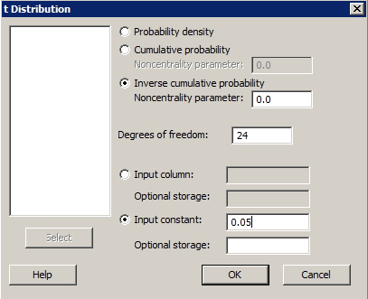
Sample Minitab Output
Inverse Cumulative Distribution Function
Student's t distribution with 24 DF
| P ( X ≤ x) | x |
|---|---|
| 0.05 | -1.71088 |
Video Review
Find a t-based P-value
Find a t-based P-valueMinitab® – Procedure
You may need to find a P-value if you are using the P-value approach to conduct a hypothesis test that uses a t-statistic.
- Select Calc >> Probability Distributions >> t ...
- Click the button labeled 'Cumulative probability'.
- Type the number of degrees of freedom in the box labeled 'Degrees of freedom'.
- Click the button labeled 'Input constant'. In the box, type the test statistic for which you want to find the associated cumulative probability.
- Select OK. The probability that a t-distributed random variable with this number of degrees of freedom is less than or equal to the test statistic will appear in the session window.
- The P-value is this probability for a lower-tail test or one minus this probability for an upper-tail test. For a two-tail test multiply the one-tail probability by two.
Example
The US National Research Council currently recommends that females between the ages of 11 and 50 intake 15 milligrams of iron daily.
Is there evidence that the population of American females is, on average, getting less than the recommended 15 mg of iron? That is, should we reject the null hypothesis H0: μ = 15 against the alternative HA: μ < 15?
The iron intakes (irondef.txt) of a random sample of 25 such American females yielded a t-statistic of -1.48.
If we were interested in calculating the test at the α = 0.05 level, what is the appropriate P-value to which we should compare the t-statistic?
Minitab Dialog Box
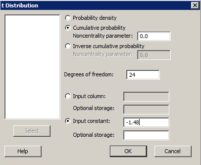
Sample Minitab Output
Cumulative Distribution Function
Student's t distribution with 24 DF
| x | P ( X ≤ x) |
|---|---|
| -1.48 | 0.0759408 |
Video Review
Find an F Critical Value
Find an F Critical ValueMinitab® – Procedure
You may need to find an F critical value if you are using the critical value approach to conduct a hypothesis test that uses an F-statistic.
- Select Calc >> Probability Distributions >> F...
- Click the button labeled Inverse cumulative probability. (Ignore the box labeled Noncentrality parameter. That is, leave the default value of 0.0 as is.)
- Type in the number of numerator degrees of freedom in the box labeled Numerator degrees of freedom.
- Type in the number of denominator degrees of freedom in the box labeled Denominator degrees of freedom.
- Click the button labeled Input Constant. In the box, type the cumulative probability for which you want to find the associated F-value.
- Select OK. The F-value will appear in the session window.
Example
Some researchers at UCLA conducted a study on cyanotic heart disease in children. They measured the age at which the child spoke his or her first word (x, in months) and the Gesell adaptive score (y) on a sample of 21 children.
Is there evidence of a relationship between age at first word and Gesell adaptive score? That is, should we reject the null hypothesis H0: β1 = 0 against the alternative hypothesis HA: β1 ≠ 0 at the 0.05 level? The resulting data (adaptive.txt) yield an ANOVA F-statistic of 13.20.
Minitab Dialog Box
Because the F-test is large regardless of whether the population slope is positive or negative, the F-test is always a one-sided test. Therefore, because we want to conduct the hypothesis test at the 0.05 level, the appropriate cumulative probability to enter is 0.95. The number of numerator degrees of freedom is always 1 for a simple linear regression model with one predictor. Because there are 21 measurements in the sample, the appropriate number of denominator degrees of freedom is 19. Therefore, your Minitab dialog box should look like:
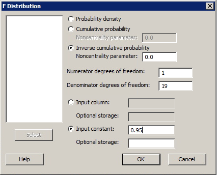
Sample Minitab Output
In this case, Minitab tells us that the F-critical value is:
Inverse Cumulative Distribution Function
F distribution with 1 DF in numerator and 19 DF in denominator
| P ( X ≤ x) | x |
|---|---|
| 0.95 | 4.38075 |
Video Review
Find an F-based P-value
Find an F-based P-valueMinitab® – Procedure
You may need to find a P-value if you are using the P-value approach to conduct a hypothesis test that uses an F-statistic.
- Select Calc >> Probability Distributions >> F ...
- Click the button labeled Cumulative probability. (Leave the non centrality parameter set as the default of 0.)
- Type the number of numerator degrees of freedom in the box labeled Numerator degrees of freedom, and type the number of the denominator degrees of freedom in the box labeled Denominator degrees of freedom.
- Click the button labeled Input constant. In the box, type the value of your F-statistic for which you want to find the associated cumulative probability.
- Select OK. The cumulative probability will appear in the session window. The P-value is 1 minus the reported cumulative probability.
Example
The coolhearts.txt data set contains the following data on 32 rabbits subjected to a heart attack:
- yi is the size of the infarcted area (in grams) of rabbit i
- xi1 is the size of the region at risk (in grams) of rabbit i
- xi2 = 1 if early cooling of rabbit i, 0 if not
- xi3 = 1 if late cooling of rabbit i, 0 if not
It can be shown that the partial F-statistic for testing H0 : β2 = β3 = 0 is 8.59 with 2 numerator and 28 denominator degrees of freedom. Find the F-based P-value so that you can draw a conclusion about the hypothesis.
Minitab Dialog Box
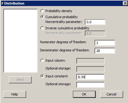
Sample Minitab Output
Cumulative Distribution Function
F distribution with 1 DF in numerator and 28 DF in denominator
| x | P ( X ≤ x) |
|---|---|
| 8.59 | 0.998767 |
The P-value is therefore 1 - 0.9988 or 0.0012.
Video Review
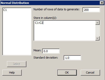
Generate Random Normally Distributed Data
Generate Random Normally Distributed DataMinitab® – Procedure
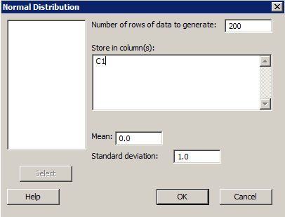
Minitab can be used to generate random data. In this example, we use Minitab to create a random set of data that is normally distributed.
- Select Calc >> Random Data >> Normal...
- In the box labeled Generate ... rows of data, type in the number of rows of data that you would like to generate.
- In the box labeled Store in Column(s):, enter the column name(s) where you want Minitab to store the data.
- In the boxes labeled Mean: and Standard deviation: type in the mean and standard deviation of your desired normal distribution. The default is the standard normal distribution with mean = 0 and standard deviation = 1.
- Select OK. The new data will appear in the worksheet window.
Example
First, generate a column of 200 random numbers from a standard normal distribution with a mean of 0 and a standard deviation of 1. Then, generate 20 more columns, each containing 200 random numbers from a standard normal distribution with a mean of 0 and a standard deviation of 1.
Minitab Dialog Boxes
First option - one column:
Second method - multiple columns:
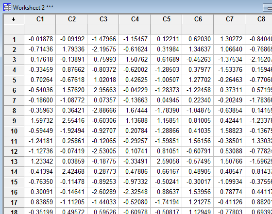
Resulting Minitab Worksheet
Based on the first dialog box above, one column (C1) of (standard) normally distributed data appears in the worksheet:
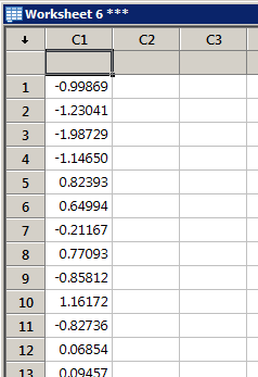 ...
...
Results based on specifying 20 columns (C1-C20) of (standard) normally distributed data as it will appear in the worksheet:
Video Review
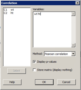
Obtain a Sample Correlation
Obtain a Sample CorrelationMinitab® – Procedure
- Select Stat >> Basic statistics >> Correlation ...
- Specify the two (or more) variables for which you want the correlation coefficient(s) calculated.
- Pearson correlation is the default. An optional Spearman rho method is also available.
- If it isn't already checked, put a checkmark in the box labeled Display p-values by clicking once on the box.
- Select OK. The output will appear in the session window.
Example
For people of the same age and gender, height is often considered a good predictor of weight. The data set htwtmales.txt contains the heights (ht, in cm) and weights (wt, in kg) of a sample of 14 males between the ages of 19 and 26 years.
- What is the sample correlation coefficient between ht and wt?
- Is there sufficient evidence to conclude that the population correlation coefficient between ht and wt is significantly different from 0?
Minitab Dialog Box
Resulting Sample Minitab Output
Correlation: wt, ht
Pearson correlation of wt and ht = 0.689
P-Value = 0.006
Video Review
Perform a Basic Regression Analysis
Perform a Basic Regression AnalysisMinitab® – Procedure
The "basic regression analysis" command outputs:
- the estimated regression function
- a table of estimated coefficients (Coef), which also includes standard errors of the coefficients (SE Coef), and t-statistics (T) and P-values (P) for testing the parameters differ from 0
- the coefficient of determination r2
- the analysis of variance table
- a table of unusual observations
- Select Stat >> Regression >> Regression >> Fit Regression Model ...
- In the box labeled "Response", specify the desired response variable.
- In the box labeled "Predictors", specify the desired predictor variable.
- Select OK. The basic regression analysis output will be displayed in the session window.
Regression Through the Origin
To fit an RTO model click "Model" in the regular regression window and uncheck "Include the constant term in the model".
Example
Sports Illustrated published results of a study designed to determine how well professional golfers putt. The data set puttgolf.txt contains data on the lengths of putts and the percentage of successful putts made by professional golfers during 15 tournaments. Only putts that were 2 to 20 feet from the hole are included in the data set.
Is there a significant linear relationship between the response y = success and the predictor x = length?
Minitab Basic Regression Analysis Dialog Box
Sample Output
Regression Analysis: success versus length
| Analysis of Variance | |||||
|---|---|---|---|---|---|
| Source | DF | Adj SS | Adj MS | F-Value | P-Value |
| Regression | 1 | 9529 | 9529.29 | 113.28 | 0.000 |
| length | 1 | 9529 | 9529.29 | 113.28 | 0.000 |
| Error | 17 | 1430 | 84.12 | ||
| Total | 18 | 10959 | |||
| Model Summary | |||||
| S | R-sq | R-sq (adj) | R-sq(pred) | ||
| 9.17166 | 86.95% | 86.18% | 82.51% | ||
|
Regression Equation success = 83.61 - 4.089 length |
|||||
| Fits and Diagnostics for Unusual Observations | |||||
| Obs | success | Fit | Resid | Std Resid |
R |
| 1 | 93.30 | 75.43 | 17.87 | 2.17 | |
| R Large residual | |||||
Video Review
Perform a Linear Regression Analysis
Perform a Linear Regression AnalysisMinitab®
- Select Stat >> Regression >> Regression >> Fit Regression Model ...
- Specify the response and the predictor(s).
- (For standard residual plots) Under Graphs..., select the desired residual plots.
- Minitab automatically recognizes replicates of data and produces the Lack of Fit test with Pure error by default.
- Select OK.
Next, back up to the Main Menu having just run this regression:
- (To get a prediction interval) Select Stat >> Regression >> Regression >> Predict ...
- Specify the response.
- Specify either the x value ("Enter individual values") or a column name ("Enter columns of values") containing multiple x values.
- Select Options... Specify the Confidence level — the default is 95%. Select OK.
- Select OK. The output will be displayed in the session window.
Regression Through the Origin
To fit an RTO model click "Model" and uncheck "Include the constant term in the model".
Example
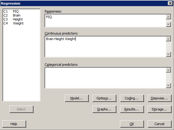
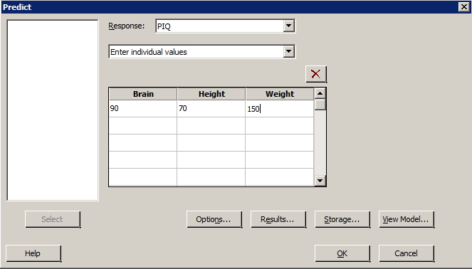
The iqsize.txt data set contains data on the IQ (y = PIQ), brain size (x1 = Brain), height (x2 = Height), and weight (x3 = Weight) of n = 38 college students. Fit the multiple linear regression model treating PIQ as the response, and Brain, Height, and Weight as the predictors. In doing so, request a lack of fit test. Also, with 95% confidence, predict the PIQ of a randomly selected college student whose Brain = 90, Height = 70 and Weight = 150.
Minitab Dialog Boxes
Resulting Minitab Output
Regression Analysis: PIQ versus Brain, Height, Weight
| Analysis of Variance | |||||
|---|---|---|---|---|---|
| Source | DF | Adj SS | Adj MS | F-Value | P-Value |
| Regression | 3 | 5572.7 | 1857.58 | 4.74 | 0.007 |
| Brain | 1 | 5239.2 | 5239.23 | 13.37 | 0.001 |
| Height | 1 | 1934.7 | 1934.71 | 4.94 | 0.033 |
| Weight | 1 | 0.0 | 0.0 | 0.00 | 0.998 |
| Error | 34 | 13321.8 | 391.82 | ||
| Total | 37 | 18894.6 | |||
| Model Summary | |||||
| S | R-sq | R-sq (adj) | R-sq(pred) | ||
| 19.7944 | 29.49% | 23.27% | 12.76% | ||
| Coefficients | |||||
| Term | Coef | SE Coef | T-Value | P-Value | VIF |
| Constant | 111.4 | 63.0 | 1.77 | 0.086 | |
| Brain | 2.060 | 0.563 | 3.66 | 0.001 | 1.58 |
| Height | -2.73 | 1.23 | -2.22 | 0.033 | 2.28 |
| Weight | 0.001 | 0.197 | 0.00 | 0.998 | 2.02 |
|
Regression Equation PIQ = 111.4 + 2.060 Brain - 2.73 Height + 0.001 Weight |
|||||
| Fits and Diagnostics for Unusual Observations | |||||
| Obs | PIQ | Fit | Resid | Std Resid |
R |
| 13 | 147.00 | 95.31 | 51.69 | 2.72 | |
| R Large residual | |||||
| Prediction for PIQ | |||||
|
Regression Equation PIQ = 111.4 + 2.060 Brain - 2.73 Height + 0.001 Weight |
|||||
| Variable | Setting | no heading | |||
| Brain | 90 | ||||
| Height | 70 | ||||
| Fit | SE Fit | 95% CI | 95% PI | ||
| 105.636 | 3.90554 | (97.6986, 113.573) | (64.6330, 146.638) | ||
Video Review
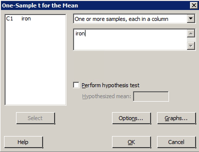
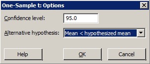
Perform a t-test for a Population Mean µ
Perform a t-test for a Population Mean µMinitab® – Procedure
- Select Stat >> Basic Statistics >> 1 Sample t ...
- If it is not already done so, use the pull-down options to select, 'Samples in columns'.
- Select the variable you want to analyze by clicking or by highlighting and clicking once on 'Select', so it appears in the box labeled 'Samples in columns'.
- In the box labeled 'Test mean', type the assumed value of the mean under the null hypothesis.
- Select Options ... (Ignore the box labeled 'Confidence level'.) For the box labeled 'Alternative', use the pull-down options to select the direction of the alternative hypothesis (less than, not equal, greater than).
- Select OK.
- Select OK. The output will appear in the session window.
Example
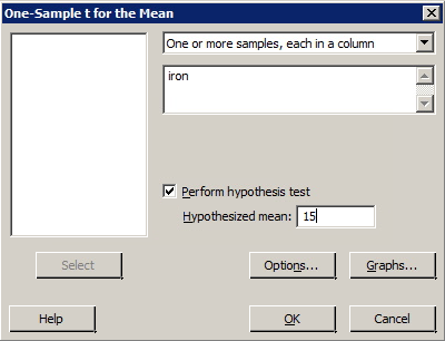
The US National Research Council currently recommends that females between the ages of 11 and 50 intake 15 milligrams of iron daily. The iron intakes of a random sample of 25 such American females are found in the dataset irondef.txt. Is there evidence that the population of American females is, on average, getting less than the recommended 15 mg of iron? That is, should we reject the null hypothesis H0: μ = 15 against the alternative HA: μ < 15? Using Minitab, determine a 95% confidence interval for μ, the mean iron intake of all women in the population.
Minitab Dialog Boxes
Sample Minitab Output
One-Sample T: iron
Test of \(\mu=15 \text { vs }<15\)
| Variable | N | Mean | StDev | SE Mean | 95% Upper Bound | T | P |
|---|---|---|---|---|---|---|---|
| iron | 25 | 14.300 | 2.367 | 0.473 | 15.110 | -1.48 | 0.076 |
Video Review
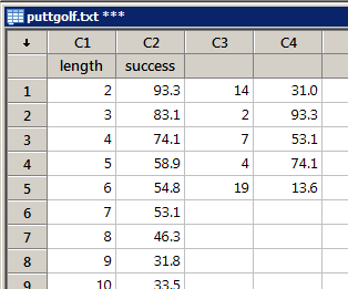
Randomly Sample Data with Replacement from Columns
Randomly Sample Data with Replacement from ColumnsMinitab® – Procedure
Random sampling from a data set allows one to analyze a subset of the data rather than the entire data set. When you randomly sample "with replacement," you allow the same data point to be selected more than once. Sampling as such helps to ensure that the selected data points are independent.
- Select Calc >> Random data >> Sample from columns...
- In the box labeled "From columns:", specify the number of data points you want to sample.
- In the larger box under the "Sample ... rows from columns" label, specify from which (two) columns you want to sample.
- In the box labeled "Store samples in...", specify two unused columns to store your selected data points.
- Select (put a checkmark in) the box labeled "Sample with replacement."
- Select OK. The randomly sampled data points will appear in the worksheet.
Example
Sports Illustrated published results of a study designed to determine how well professional golfers putt. The data set puttgolf.txt contains data on the lengths of putts and the percentage of successful putts made by professional golfers during 15 tournaments. Only putts that were 2 to 20 feet from the hole are included in the data set.
Randomly sample 5 golfers (with replacement) from the data set.
Minitab Sample from Columns Dialog Box
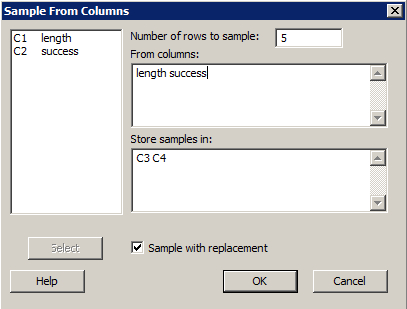
Sample Random Selection of 5 Data Points
Video Review
Split the Worksheet Based on the Value of a Variable
Split the Worksheet Based on the Value of a VariableMinitab® – Procedure
- Select Data >> Split Worksheet...
- In the box labeled By variables, specify the variable based on which you want the worksheet to be split.
- Select OK. The new worksheets, based on the original worksheet, will appear.
Example
A laboratory tested the relationship between operating cost per mile (y = cost) and cruising speed (x = speed) for two different makes (0, 1) of truck tires. The resulting data are stored in tiretesting.txt (Neter, Kutner, et al, 1996, p. 493). Split the worksheet into two worksheets based on the value of the variable make.
Minitab Dialog Box
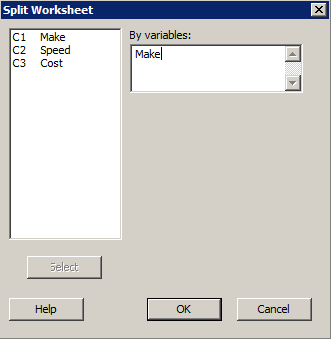
Resulting Sample Minitab Output
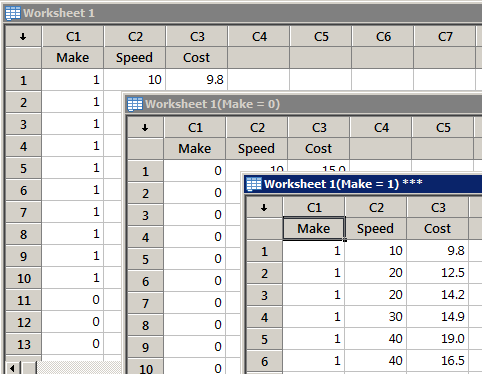
Worksheet is split into two worksheets; one for each make of truck.
Video Review
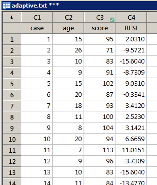
Store Residuals, Leverages, and Influence Measures
Store Residuals, Leverages, and Influence MeasuresMinitab® – Procedure
- Select Stat >> Regression >> Regression >> Fit Regression Model ...
- Specify the response and the predictor variable(s).
- Select Storage... Under Diagnostic Measures, select the type of residuals (and/or influence measures) that you want to be stored. Select OK.
- Select OK. The requested residuals (and/or influence measures) will be stored in your worksheet.
Example
The data set adaptive.txt contains the Gesell adaptive scores and ages (in months) of n = 21 children with cyanotic heart disease. Upon regressing the response y = score on the predictor x = age, store the resulting standardized residuals in the worksheet.
Minitab Dialog Boxes
Minitab Worksheet with a New Column of Stored Residuals