
To introduce the idea of variability, consider this example. Two vending machines A and B drop candies when a quarter is inserted. The number of pieces of candy one gets is random. The following data are recorded for six trials at each vending machine:
Pieces of candy from vending machine A:
1, 2, 3, 3, 5, 4
mean = 3, median = 3, mode = 3
Pieces of candy from vending machine B:
2, 3, 3, 3, 3, 4
mean = 3, median = 3, mode = 3
The dot plot for the pieces of candy from vending machine A and vending machine B is displayed in figure 1.4.
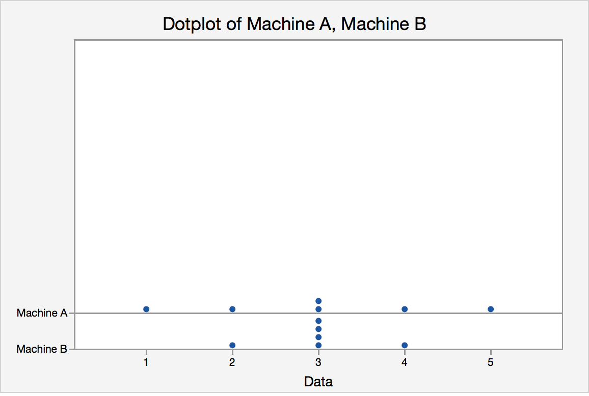
They have the same center, but what about their spreads?
Measures of Variability
There are many ways to describe variability or spread including:
- Range
- Interquartile range (IQR)
- Variance and Standard Deviation
- Range
- The range is the difference in the maximum and minimum values of a data set. The maximum is the largest value in the dataset and the minimum is the smallest value. The range is easy to calculate but it is very much affected by extreme values.
- \(Range = maximum - minimum\)
Like the range, the IQR is a measure of variability, but you must find the quartiles in order to compute its value.
- Interquartile Range (IQR)
- The interquartile range is the difference between upper and lower quartiles and denoted as IQR.
- \begin{align} IQR &=Q3 -Q1\\&=upper\ quartile - lower\ quartile\\&= 75th\ percentile - 25th\ percentile \end{align}
Try it! Section
Find the IQR for the final exam scores example.
Variance and Standard Deviation Section
One way to describe spread or variability is to compute the standard deviation. In the following section, we are going to talk about how to compute the sample variance and the sample standard deviation for a data set. The standard deviation is the square root of the variance.
- Variance
- the average squared distance from the mean
- Population variance
- \(\sigma^2=\dfrac{\sum_{i=1}^N (x_i-\mu)^2}{N}\)
- where $\mu$ is the population mean and the summation is over all possible values of the population and \(N\) is the population size.
$\sigma^2$ is often estimated by using the sample variance.
- Sample Variance
- \(s^2=\dfrac{\sum_{i=1}^n (x_i-\bar{x})^2}{n-1}=\dfrac{\sum_{i=1}^n x_i^2-n\bar{x}^2}{n-1}\)
- Where $n$ is the sample size and $\bar{x}$ is the sample mean.
Why do we divide by \(n-1\) instead of by \(n\)?
When we calculate the sample sd we estimate the population mean with the sample mean, and dividing by (n-1) rather than n which gives it a special property that we call an "unbiased estimator". Therefore \(s^2\) is an unbiased estimator for the population variance.
The sample variance (and therefore sample standard deviation) are the common default calculations used by software. When asked to calculate the variance or standard deviation of a set of data, assume - unless otherwise instructed - this is sample data and therefore calculating the sample variance and sample standard deviation.
Example 1-8 Section
Calculate the variance for these final exam scores.
24, 58, 61, 67, 71, 73, 76, 79, 82, 83, 85, 87, 88, 88, 92, 93, 94, 97
First, find the mean:
$\bar{x}=\dfrac{24+58+61+67+71+73+76+79+82+83+85+87+88+88+92+93+94+97}{18}=\dfrac{233}{3}$
|
$x_i$ |
$(x-\bar{x})$ |
$(x-\bar{x})^2$ |
|---|---|---|
|
24 |
-161/3 |
25921/9 |
|
58 |
-59/3 |
3481/9 |
|
61 |
-50/3 |
2500/3 |
|
67 |
-32/3 |
1024/9 |
|
71 |
-20/3 |
400/9 |
|
73 |
-14/3 |
196/9 |
|
76 |
-5/3 |
25/9 |
|
79 |
4/3 |
16/9 |
|
82 |
13/3 |
169/9 |
|
83 |
16/3 |
256/9 |
|
85 |
22/3 |
484/9 |
|
87 |
28/3 |
784/9 |
|
88 |
31/3 |
961/9 |
|
88 |
31/3 |
961/9 |
|
92 |
43/3 |
1849/9 |
|
93 |
46/3 |
2116/9 |
|
94 |
49/3 |
2401/9 |
|
97 |
58/3 |
3364/9 |
|
Sum |
0 |
46908/9 |
Finally,
\(s^2=\dfrac{\sum_{i=1}^n (x_i-\bar{x})^2}{18-1}=\dfrac{46908/9}{17}=\dfrac{5212}{17}\approx 306.588\)
Try it! Section
Calculate the sample variances for the data set from vending machines A and B yourself and check that it the variance for B is smaller than that for data set A. Work out your answer first, then click the graphic to compare answers.
\(\bar{y}_A=\dfrac{1}{6}(1+2+3+3+5+4)=\dfrac{18}{6}=3\)
\(s^2_A=\dfrac{(1-3)^2+(2-3)^2+(3-3)^2+(3-3)^2+(4-3)^2+(5-3)^2}{6-1}=2\)
\(\bar{y}_B=\dfrac{1}{6}(2+3+3+3+3+4)=\dfrac{18}{6}=3\)
\(s^2_B=\dfrac{(2-3)^2+(3-3)^2+(3-3)^2+(3-3)^2+(3-3)^2+(4-3)^2}{6-1}=0.4\)
Standard Deviation Section
The standard deviation is a very useful measure. One reason is that it has the same unit of measurement as the data itself (e.g. if a sample of student heights were in inches then so, too, would be the standard deviation. The variance would be in squared units, for example \(inches^2\)). Also, the empirical rule, which will be explained later, makes the standard deviation an important yardstick to find out approximately what percentage of the measurements fall within certain intervals.
- Standard Deviation
- approximately the average distance the values of a data set are from the mean or the square root of the variance
- Population Standard deviation
- \(\sigma=\sqrt{\sigma^2}\)
It has the same unit as the \(x_i\)’s. This is a desirable property since one may think about the spread in terms of the original unit.
\(\sigma\) is estimated by the sample standard deviation \(s\) :
- Sample Standard Deviation
- \(s=\sqrt{s^2}\)
A rough estimate of the standard deviation can be found using \(s\approx \frac{\text{range}}{4}\)
Adding and Multiplying Constants
What happens to measures of variability if we add or multiply each observation in a data set by a constant? We learned previously about the effect such actions have on the mean and the median, but do variation measures behave similarly? Not really.
When we add a constant to all values we are basically shifting the data upward (or downward if we subtract a constant). This has the result of moving the middle but leaving the variability measures (e.g. range, IQR, variance, standard deviation) unchanged.
On the other hand, if one multiplies each value by a constant this does affect measures of variation. The result on the variance is that the new variance is multiplied by the square of the constant, while the standard deviation, range, and IQR are multiplied by the constant. For example, if the observed values of Machine A in the example above were multiplied by three, the new variance would be 18 (the original variance of 2 multiplied by 9). The new standard deviation would be 4.242 (the original standard 1.414 multiplied by 3). The range and IQR would also change by a factor of 3.
Coefficient of Variation
Above we considered three measures of variation: Range, IQR, and Variance (and its square root counterpart - Standard Deviation). These are all measures we can calculate from one quantitative variable e.g. height, weight. But how can we compare dispersion (i.e. variability) of data from two or more distinct populations that have vastly different means?
A popular statistic to use in such situations is the Coefficient of Variation or CV. This is a unit-free statistic and one where the higher the value the greater the dispersion. The calculation of CV is:
- Coefficient of Variation (CV)
- \(CV = \dfrac{\text{Standard Deviation}}{\text{Mean}}\)
To demonstrate, think of prices for luxury and budget hotels. Which do you think would have the higher average cost per night? Which would have the greater standard deviation? The CV would allow you to compare this dispersion in costs in relative terms by accounting for the fact that the luxury hotels would have a greater mean and standard deviation.
Example 1-9: Comparing Prices Section
You are shopping for toilet tissue. As you compare prices of various brands, some offer price per roll while others offer price per sheet. You are interested in determining which pricing method has less variability so you sample several of each and calculate the mean and standard deviation for the sampled items that are priced per roll, and the mean and standard deviation for the sampled items that are priced per sheet. The table below summarizes your results.
|
Item |
Mean |
Standard Deviation |
|---|---|---|
|
Price per Roll |
0.9196 |
0.4233 |
|
Price Per Sheet |
0.01134 |
0.00553 |
Comparing the standard deviations the Per Sheet appears to have much less variability in pricing. However, the mean is also much smaller. The coefficient of variation allows us to make a relative comparison of the variability of these two pricing schemes:
\(CV_{roll}=\dfrac{0.4233}{0.9196}=0.46\)
\(CV_{sheet}=\dfrac{0.00553}{0.01134}=0.49\)
Relatively speaking, the variation for Price per Sheet is greater than the variability for Price per Roll.