
A binary variable is a variable that has two possible outcomes. For example, sex (male/female) or having a tattoo (yes/no) are both examples of a binary categorical variable.
A random variable can be transformed into a binary variable by defining a “success” and a “failure”. For example, consider rolling a fair six-sided die and recording the value of the face. The random variable, value of the face, is not binary. If we are interested, however, in the event A={3 is rolled}, then the “success” is rolling a three. The failure would be any value not equal to three. Therefore, we can create a new variable with two outcomes, namely A = {3} and B = {not a three} or {1, 2, 4, 5, 6}. This new variable is now a binary variable.
Binary Categorical Variable
A binary categorical variable is a variable that has two possible outcomes.
The Binomial Distribution
The binomial distribution is a special discrete distribution where there are two distinct complementary outcomes, a “success” and a “failure”.
We have a binomial experiment if ALL of the following four conditions are satisfied:
- The experiment consists of n identical trials (n is fixed).
- Each trial results in one of the two outcomes, called success and failure.
- The probability of success, denoted p, remains the same from trial to trial.
- The n trials are independent. That is, the outcome of any trial does not affect the outcome of the others.
If the four conditions are satisfied, then the random variable \(X\)=number of successes in \(n\) trials, is a binomial random variable with
\begin{align}
&\mu=E(X)=np &&\text{(Mean)}\\
&\text{Var}(X)=np(1-p) &&\text{(Variance)}\\
&\text{SD}(X)=\sqrt{np(1-p)} \text{, where \(p\) is the probability of the “success."} &&\text{(Standard Deviation)}\\
\end{align}
A Note on Notation! Some common notation for “success” that you may see will be either \(p\) or \(\pi\) to represent the probability of “success” and usually \(q=1-p\) to represent the probability of “failure”. \(\pi\) is what is used in text. “Success” is defined as whatever the researcher decides…not just a positive outcome. The symbol \(\pi\) is this case does NOT refer the numerical value 3.14
\(p \;(or\ \pi)\) = probability of success
Example 3-5: Prior Convictions Section
Let's use the example from the previous page investigating the number of prior convictions for prisoners at a state prison at which there were 500 prisoners. Define the “success” to be the event that a prisoner has no prior convictions. Find \(p\) and \(1-p\).
Answer
Let Success = no priors (0)
Let Failure = priors (1, 2, 3, or 4)
Looking back on our example, we can find that:
\(p=0.16\)
\(1-p=1-0.16=0.84\)
Verify by \(p+(1-p)=1\)
Example 3-6: Crime Survey Section
An FBI survey shows that about 80% of all property crimes go unsolved. Suppose that in your town 3 such crimes are committed and they are each deemed independent of each other. What is the probability that 1 of 3 of these crimes will be solved?
First, we must determine if this situation satisfies ALL four conditions of a binomial experiment:
- Does it satisfy a fixed number of trials? YES the number of trials is fixed at 3 (n = 3.)
- Does it have only 2 outcomes? YES (Solved and unsolved)
- Do all the trials have the same probability of success? YES (p = 0.2)
- Are all crimes independent? YES (Stated in the description.)
To find the probability that only 1 of the 3 crimes will be solved we first find the probability that one of the crimes would be solved. With three such events (crimes) there are three sequences in which only one is solved:
- Solved First, Unsolved Second, Unsolved Third = (0.2)(0.8)( 0.8) = 0.128
- Unsolved First, Solved Second, Unsolved Third = (0.8)(0.2)(0.8) = 0.128
- Unsolved First, Unsolved Second, Solved Third = (0.8)(0.8)(0.2) = 0.128
We add these 3 probabilities up to get 0.384. Looking at this from a formula standpoint, we have three possible sequences, each involving one solved and two unsolved events. Putting this together gives us the following: \(3(0.2)(0.8)^2=0.384\)
The example above and its formula illustrates the motivation behind the binomial formula for finding exact probabilities.
The Binomial Formula
For a binomial random variable with probability of success, \(p\), and \(n\) trials...
\(f(x)=P(X = x)=\dfrac{n!}{x!(n−x)!}p^x(1–p)^{n-x}\) for \(x=0, 1, 2, …, n\)
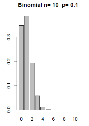
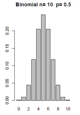
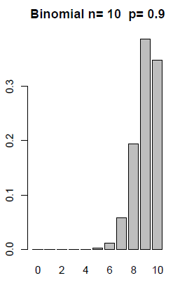
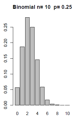
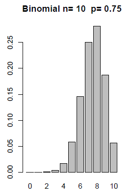
Graphical Displays of Binomial Distributions Section
The formula defined above is the probability mass function, pmf, for the Binomial. We can graph the probabilities for any given \(n\) and \(p\). The following distributions show how the graphs change with a given n and varying probabilities.
Example 3-7: Crime Survey Continued... Section
For the FBI Crime Survey example, what is the probability that at least one of the crimes will be solved?
Answer
Here we are looking to solve \(P(X \ge 1)\).
There are two ways to solve this problem: the long way and the short way.
The long way to solve for \(P(X \ge 1)\). This would be to solve \(P(x=1)+P(x=2)+P(x=3)\) as follows:
\(P(x=1)=\dfrac{3!}{1!2!}0.2^1(0.8)^2=0.384\)
\(P(x=2)=\dfrac{3!}{2!1!}0.2^2(0.8)^1=0.096\)
\(P(x=3)=\dfrac{3!}{3!0!}0.2^3(0.8)^0=0.008\)
We add up all of the above probabilities and get 0.488...OR...we can do the short way by using the complement rule. Here the complement to \(P(X \ge 1)\) is equal to \(1 - P(X < 1)\) which is equal to \(1 - P(X = 0)\). We have carried out this solution below.
\begin{align} 1–P(x<1)&=1–P(x=0)\\&=1–\dfrac{3!}{0!(3−0)!}0.2^0(1–0.2)^3\\ &=1−1(1)(0.8)^3\\ &=1–0.512\\ &=0.488 \end{align}
In such a situation where three crimes happen, what is the expected value and standard deviation of crimes that remain unsolved? Here we apply the formulas for expected value and standard deviation of a binomial.
\begin{align} \mu &=E(X)\\ &=3(0.8)\\ &=2.4 \end{align} \begin{align} \text{Var}(X)&=3(0.8)(0.2)=0.48\\ \text{SD}(X)&=\sqrt{0.48}\approx 0.6928 \end{align}
Note: X can only take values 0, 1, 2, ..., n, but the expected value (mean) of X may be some value other than those that can be assumed by X.
Example 3-8: Cross-Fertilizing Section
Cross-fertilizing a red and a white flower produces red flowers 25% of the time. Now we cross-fertilize five pairs of red and white flowers and produce five offspring. Find the probability that there will be no red-flowered plants in the five offspring.
Answer
Y = # of red flowered plants in the five offspring. Here, the number of red-flowered plants has a binomial distribution with \(n = 5, p = 0.25\).
\begin{align} P(Y=0)&=\dfrac{5!}{0!(5−0)!}p^0(1−p)^5\\&=1(0.25)^0(0.75)^5\\&=0.237 \end{align}
Try it! Section
Refer to example 3-8 to answer the following.
- Find the probability that there will be four or more red-flowered plants.
\begin{align} P(\mbox{Y is 4 or more})&=P(Y=4)+P(Y=5)\\ &=\dfrac{5!}{4!(5-4)!} {p}^4 {(1-p)}^1+\dfrac{5!}{5!(5-5)!} {p}^5 {(1-p)}^0\\ &=5\cdot (0.25)^4 \cdot (0.75)^1+ (0.25)^5\\ &=0.015+0.001\\ &=0.016\\ \end{align}
- Of the five cross-fertilized offspring, how many red-flowered plants do you expect?\begin{align} \mu &=5⋅0.25\\&=1.25 \end{align}
- What is the standard deviation of Y, the number of red-flowered plants in the five cross-fertilized offspring?\begin{align} \sigma&=\sqrt{5\cdot0.25\cdot0.75}\\ &=0.97 \end{align}