
In 1908, William Sealy Gosset from Guinness Breweries discovered the t-distribution. His pen-name was Student and thus it is called the "Student's t-distribution."
The t-distribution is different for different sample size, n. Thus, tables, as detailed as the standard normal table, are not provided in the usual statistics books. The graph below shows the t-distribution for degrees of freedom of 10 (blue) and 30 (red dashed).
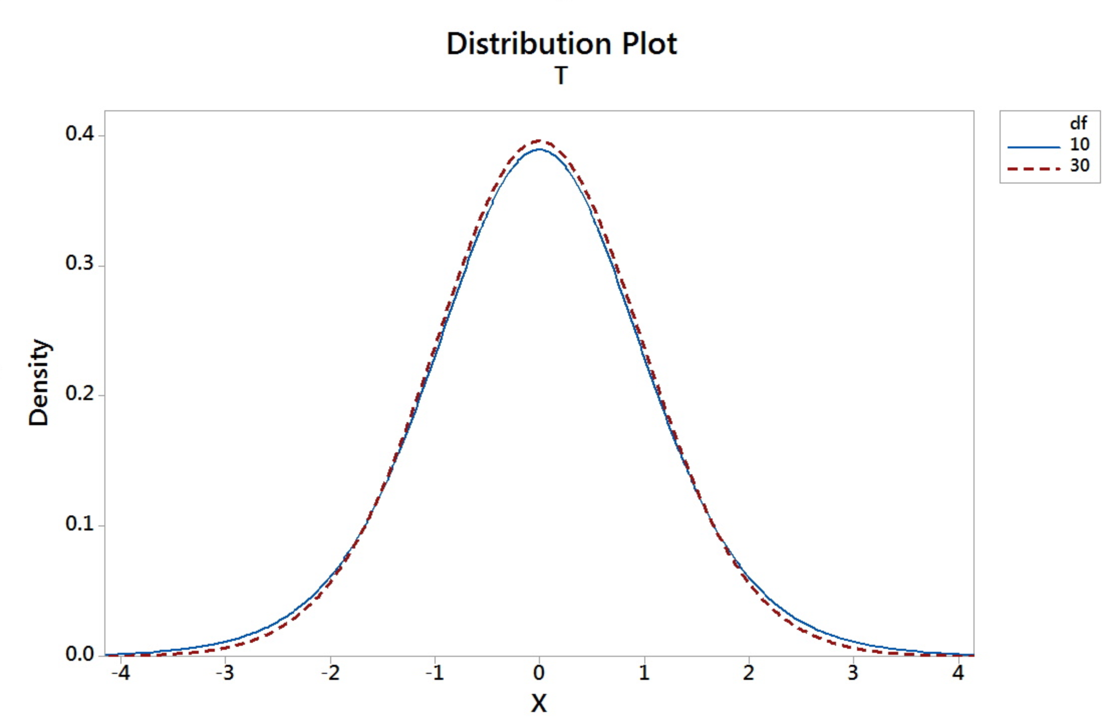
Properties of the t-distribution
- t is symmetric about 0
- t-distribution is more variable than the Standard Normal distribution
- t-distributions are different for different degrees of freedom (d.f.).
- The larger $n$ gets (or as $n$ goes to infinity), the closer the $t$-distribution is to the $z$.
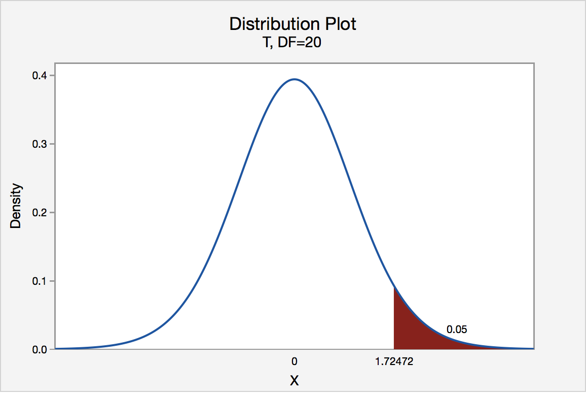
- The meaning of $t_\alpha$ is the $t$-value having the area "$\alpha$" to the right of it.
Example 5-5: Finding t-values Section
Use this t-table or the one in your text to find following the example.
Find \(t_{0.05}\) where the degree of freedom is 20.
In a t-distribution table below the top row represents the upper tail area, while the first column are the degrees of freedom.
The \(t_{0.05}\) where the degree of freedom is 20 is 1.725 .
| df | 0.40 | 0.25 | 0.10 | 0.05 | 0.025 | 0.01 | 0.005 | 0.001 | .0005 |
|---|---|---|---|---|---|---|---|---|---|
| ... | ... | ... | ... | ... | ... | ... | ... | ... | ... |
| 18 | 0.257 | 0.688 | 1.330 | 1.734 | 2.101 | 2.552 | 2.878 | 3.610 | 3.922 |
| 19 | 0.257 | 0.688 | 1.328 | 1.729 | 2.093 | 2.539 | 2.861 | 3.579 | 3.883 |
| 20 | 0.257 | 0.687 | 1.325 | 1.725 | 2.086 | 2.528 | 2.845 | 3.552 | 3.850 |
| 21 | 0.257 | 0.686 | 1.323 | 1.721 | 2.080 | 2.518 | 2.831 | 3.527 | 3.819 |
The graph shows that the \(\alpha\) values at the top of this table are the upper tail areas of the distribution.
Find \(t_{0.05}\) where the degree of freedom is 34.
What do we do when the degrees of freedom are not on the table? The t-table degrees of freedom run continuously from 1 to 30, then go by intervals after 30 (e.g. after 30 we have 35). In such cases, we can use software such as Minitab to find a more exact value for the multiplier as opposed to using a degrees of freedom that is "close".
To find the t-value in Minitab...
- From the Minitab Menu select Calc > Probability Distributions > t...
- Choose inverse cumulative probability
- Enter the degrees of freedom
- Set the input constant as 0.95 (1 - 0.05).
- Choose OK
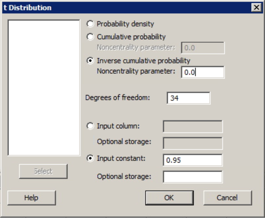
The output from Minitab gives us \(t_{0.05}\) with df= 34 as 1.69092.
| P (X \(\le\) x) | x |
|---|---|
| 0.95 | 1.69092 |
The t-value for an \(\alpha\) of .05 and df of 30 is 1.697.
| df | 0.40 | 0.25 | 0.10 | 0.05 | 0.025 | 0.01 | 0.005 | 0.001 | .0005 |
|---|---|---|---|---|---|---|---|---|---|
| ... | ... | ... | ... | ... | ... | ... | ... | ... | ... |
| 27 | 0.256 | 0.684 | 1.314 | 1.703 | 2.052 | 2.473 | 2.771 | 3.421 | 3.690 |
| 28 | 0.256 | 0.683 | 1.313 | 1.701 | 2.048 | 2.467 | 2.763 | 3.408 | 3.674 |
| 29 | 0.256 | 0.683 | 1.311 | 1.699 | 2.045 | 2.462 | 2.756 | 3.396 | 3.659 |
| 30 | 0.256 | 0.683 | 1.310 | 1.697 | 2.042 | 2.457 | 2.750 | 3.385 | 3.646 |
Note! When the sample size is larger than 30, the t-values are not that different from the z-values. Thus, a crude estimate for \(t_{0.05}\) with 34 degrees of freedom is \(z_{0.05} = 1.645\). Although it is a crude estimate, when software is available, it is best to find the $t$ values rather than use the $z$.