
Introduction Section
When we developed the inference for the independent samples, we depended on the statistical theory to help us. The theory, however, required the samples to be independent. What can we do when the two samples are not independent, i.e., the data is paired?
Consider an example where we are interested in a person’s weight before implementing a diet plan and after. Since the interest is focusing on the difference, it makes sense to “condense” these two measurements into one and consider the difference between the two measurements. For example, if instead of considering the two measures, we take the before diet weight and subtract the after diet weight. The difference makes sense too! It is the weight lost on the diet.
When we take the two measurements to make one measurement (i.e., the difference), we are now back to the one sample case! Now we can apply all we learned for the one sample mean to the difference (Cool!)
The Confidence Interval for the Difference of Paired Means, \(\mu_d\) Section
When we consider the difference of two measurements, the parameter of interest is the mean difference, denoted \(\mu_d\). The mean difference is the mean of the differences. We are still interested in comparing this difference to zero.
Suppose we have two paired samples of size \(n\):
\(x_1, x_2, …., x_n\) and \(y_1, y_2, … , y_n\)
Their difference can be denoted as:
\(d_1=x_1-y_1, d_2=x_2-y_2, …., d_n=x_n-y_n\)
The sample mean of the differences is:
\(\bar{d}=\frac{1}{n}\sum_{i=1}^n d_i\)
Denote the sample standard deviation of the differences as \(s_d\).
If \(\bar{d}\) is normal (or the sample size is large), the sampling distribution of \(\bar{d}\) is (approximately) normal with mean \(\mu_d\), standard error \(\dfrac{\sigma_d}{\sqrt{n}}\), and estimated standard error \(\dfrac{s_d}{\sqrt{n}}\).
At this point, the confidence interval will be the same as that of one sample.
- \(\boldsymbol{(1-\alpha)100\%}\) Confidence interval for \(\boldsymbol{\mu_d}\)
-
\(\bar{d}\pm t_{\alpha/2}\frac{s_d}{\sqrt{n}}\)
where \(t_{\alpha/2}\) comes from \(t\)-distribution with \(n-1\) degrees of freedom
Example 7-6: Zinc Concentrations Section
Trace metals in drinking water affect the flavor and an unusually high concentration can pose a health hazard. Ten pairs of data were taken measuring zinc concentration in bottom water and surface water (zinc_conc.txt).
Does the data suggest that the true average concentration in the bottom water is different than that of surface water? Construct a confidence interval to address this question.
Zinc concentrations
| 1 | 2 | 3 | 4 | 5 | 6 | 7 | 8 | 9 | 10 | |
|---|---|---|---|---|---|---|---|---|---|---|
| Bottom Water | .430 | .266 | .567 | .531 | .707 | .716 | .651 | .589 | .469 | .723 |
| Surface Water | .415 | .238 | .390 | .410 | .605 | .609 | .632 | .523 | .411 | .612 |
In this example, the response variable is concentration and is a quantitative measurement. The explanatory variable is location (bottom or surface) and is categorical. The two populations (bottom or surface) are not independent. Therefore, we are in the paired data setting. The parameter of interest is \(\mu_d\).
Find the difference as the concentration of the bottom water minus the concentration of the surface water.
Since the problem did not provide a confidence level, we should use 5%.
To use the methods we developed previously, we need to check the conditions. The problem does not indicate that the differences come from a normal distribution and the sample size is small (n=10). We should check, using the Normal Probability Plot to see if there is any violation. First, we need to find the differences.
|
Difference |
0.015 |
0.028 |
0.177 |
0.121 |
0.102 |
0.107 |
0.019 |
0.066 |
0.058 |
0.111 |
|---|
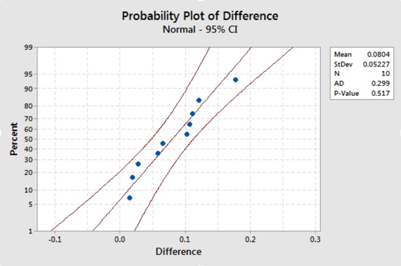
All of the differences fall within the boundaries, so there is no clear violation of the assumption. We can proceed with using our tools, but we should proceed with caution.
We need all of the pieces for the confidence interval. The sample mean difference is \(\bar{d}=0.0804\) and the standard deviation is \(s_d=0.0523\). For practice, you should find the sample mean of the differences and the standard deviation by hand. With \(n-1=10-1=9\) degrees of freedom, \(t_{0.05/2}=2.2622\).
The 95% confidence interval for the mean difference, \(\mu_d\) is:
\(\bar{d}\pm t_{\alpha/2}\dfrac{s_d}{\sqrt{n}}\)
\(0.0804\pm 2.2622\left( \dfrac{0.0523}{\sqrt{10}}\right)\)
(0.04299, 0.11781)
We are 95% confident that the population mean difference of bottom water and surface water zinc concentration is between 0.04299 and 0.11781.
If there is no difference between the means of the two measures, then the mean difference will be 0. Since 0 is not in our confidence interval, then the means are statistically different (or statistical significant or statistically different).
Note! Minitab will calculate the confidence interval and a hypothesis test simultaneously. We demonstrate how to find this interval using Minitab after presenting the hypothesis test.
Hypothesis Test for the Difference of Paired Means, \(\mu_d\) Section
In this section, we will develop the hypothesis test for the mean difference for paired samples. As we learned in the previous section, if we consider the difference rather than the two samples, then we are back in the one-sample mean scenario.
The possible null and alternative hypotheses are:
\(H_0\colon \mu_d=0\)
\(H_a\colon \mu_d\ne 0\)
\(H_a\colon \mu_d>0\)
\(H_a\colon \mu_d<0\)
We still need to check the conditions and at least one of the following need to be satisfied:
- The differences of the paired follow a normal distribution
- The sample size is large, \(n>30\).
If at least one is satisfied then...
\(t^*=\dfrac{\bar{d}-0}{\frac{s_d}{\sqrt{n}}}\)
Will follow a t-distribution with \(n-1\) degrees of freedom.
The same process for the hypothesis test for one mean can be applied. The test for the mean difference may be referred to as the paired t-test or the test for paired means.
Example 7-7: Zinc Concentrations - Hypothesis Test Section
Recall the zinc concentration example. Does the data suggest that the true average concentration in the bottom water exceeds that of surface water? Conduct this test using the rejection region approach. (zinc_conc.txt).
Zinc concentrations
| 1 | 2 | 3 | 4 | 5 | 6 | 7 | 8 | 9 | 10 | |
|---|---|---|---|---|---|---|---|---|---|---|
| Bottom Water | .430 | .266 | .567 | .531 | .707 | .716 | .651 | .589 | .469 | .723 |
| Surface Water | .415 | .238 | .390 | .410 | .605 | .609 | .632 | .523 | .411 | .612 |
If we find the difference as the concentration of the bottom water minus the concentration of the surface water, then null and alternative hypotheses are:
\(H_0\colon \mu_d=0\) vs \(H_a\colon \mu_d>0\)
Note! If the difference was defined as surface - bottom, then the alternative would be left-tailed.
The desired significance level was not stated so we will use \(\alpha=0.05\).
The assumptions were discussed when we constructed the confidence interval for this example. Remember although the Normal Probability Plot for the differences showed no violation, we should still proceed with caution.
The next step is to find the critical value and the rejection region. The critical value is the value \(a\) such that \(P(T>a)=0.05\). Using the table or software, the value is 1.8331. For a right-tailed test, the rejection region is \(t^*>1.8331\).
Recall from the previous example, the sample mean difference is \(\bar{d}=0.0804\) and the sample standard deviation of the difference is \(s_d=0.0523\). Therefore, the test statistic is:
\(t^*=\dfrac{\bar{d}-0}{\frac{s_d}{\sqrt{n}}}=\dfrac{0.0804}{\frac{0.0523}{\sqrt{10}}}=4.86\)
The value of our test statistic falls in the rejection region. Therefore, we reject the null hypothesis. With a significance level of 5%, there is enough evidence in the data to suggest that the bottom water has higher concentrations of zinc than the surface level.
Minitab® – Paired t-Test
You can use a paired t-test in Minitab to perform the test. Alternatively, you can perform a 1-sample t-test on difference = bottom - surface.
- Choose Stat> Basic Statistics> Paired t
- Click Optionsto specify the confidence level for the interval and the alternative hypothesis you want to test. The default null hypothesis is 0.
Zinc Concentrations Example
The Minitab output for paired T for bottom - surface is as follows:
Paired T for bottom - surface
|
N |
Mean |
StDev |
SE Mean |
|
|
bottom |
10 |
0.5649 |
0.1468 |
0.0464 |
|
surface |
10 |
0.4845 |
0.1312 |
0.0415 |
|
Difference |
10 |
0.0804 |
0.0523 |
0.0165 |
95% lower bound for mean difference: 0.0505
T-Test of mean difference = 0 (vs > 0): T-Value = 4.86 P-Value = 0.000
Note! In Minitab, if you choose a lower-tailed or an upper-tailed hypothesis test, an upper or lower confidence bound will be constructed, respectively, rather than a confidence interval.
Using the p-value to draw a conclusion about our example:
p-value = 0.000 < 0.05
Reject \(H_0\) and conclude that bottom zinc concentration is higher than surface zinc concentration.
Additional Notes Section
- For the zinc concentration problem, if you do not recognize the paired structure, but mistakenly use the 2-sample t-test treating them as independent samples, you will not be able to reject the null hypothesis. This demonstrates the importance of distinguishing the two types of samples. Also, it is wise to design an experiment efficiently whenever possible.
- What if the assumption of normality is not satisfied? Considering a nonparametric test would be wise.