
Derivation of the Test Section
We are now going to develop the hypothesis test for the difference of two proportions for independent samples. The hypothesis test will follow the same six steps we learned in the previous Lesson although they are not explicitly stated.
We will use the sampling distribution of \(\hat{p}_1-\hat{p}_2\) as we did for the confidence interval. One major difference in the hypothesis test is the null hypothesis and assuming the null hypothesis is true.
For a test for two proportions, we are interested in the difference. If the difference is zero, then they are not different (i.e., they are equal). Therefore, the null hypothesis will always be:
\(H_0\colon p_1-p_2=0\)
Another way to look at it is \(H_0\colon p_1=p_2\). This is worth stopping to think about. Remember, in hypothesis testing, we assume the null hypothesis is true. In this case, it means that \(p_1\) and \(p_2\) are equal. Under this assumption, then \(\hat{p}_1\) and \(\hat{p}_2\) are both estimating the same proportion. Think of this proportion as \(p^*\). Therefore, the sampling distribution of both proportions, \(\hat{p}_1\) and \(\hat{p}_2\), will, under certain conditions, be approximately normal centered around \(p^*\), with standard error \(\sqrt{\dfrac{p^*(1-p^*)}{n_i}}\), for \(i=1, 2\).
We take this into account by finding an estimate for this \(p^*\) using the two sample proportions. We can calculate an estimate of \(p^*\) using the following formula:
\(\hat{p}^*=\dfrac{x_1+x_2}{n_1+n_2}\)
This value is the total number in the desired categories \((x_1+x_2)\) from both samples over the total number of sampling units in the combined sample \((n_1+n_2)\).
Putting everything together, if we assume \(p_1=p_2\), then the sampling distribution of \(\hat{p}_1-\hat{p}_2\) will be approximately normal with mean 0 and standard error of \(\sqrt{p^*(1-p^*)\left(\frac{1}{n_1}+\frac{1}{n_2}\right)}\), under certain conditions.
Therefore,
\(z^*=\dfrac{(\hat{p}_1-\hat{p}_2)-0}{\sqrt{\hat{p}^*(1-\hat{p}^*)\left(\dfrac{1}{n_1}+\dfrac{1}{n_2}\right)}}\)
...will follow a standard normal distribution.
Finally, we can develop our hypothesis test for \(p_1-p_2\).
Null: \(H_0\colon p_1-p_2=0\)
Possible Alternatives:
\(H_a\colon p_1-p_2\ne0\)
\(H_a\colon p_1-p_2>0\)
\(H_a\colon p_1-p_2<0\)
Conditions:
\(n_1\hat{p}_1\), \(n_1(1-\hat{p}_1)\), \(n_2\hat{p}_2\), and \(n_2(1-\hat{p}_2)\) are all greater than five
The test statistic is:
\(z^*=\dfrac{\hat{p}_1-\hat{p}_2-0}{\sqrt{\hat{p}^*(1-\hat{p}^*)\left(\dfrac{1}{n_1}+\dfrac{1}{n_2}\right)}}\)
...where \(\hat{p}^*=\dfrac{x_1+x_2}{n_1+n_2}\).
The critical values, rejection regions, p-values, and decisions will all follow the same steps as those from a hypothesis test for a one sample proportion.
Example 7-2: Received $100 by Mistake Section

Let's continue with the question that was asked previously.
Males and females were asked about what they would do if they received a $100 bill by mail, addressed to their neighbor, but wrongly delivered to them. Would they return it to their neighbor? Of the 69 males sampled, 52 said “yes” and of the 131 females sampled, 120 said “yes.”
Does the data indicate that the proportions that said “yes” are different for males and females at a 5% level of significance? Conduct the test using the p-value approach.
Again, let’s define males as sample 1.
The conditions are all satisfied as we have shown previously.
The null and alternative hypotheses are:
\(H_0\colon p_1-p_2=0\) vs \(H_a\colon p_1-p_2\ne 0\)
The test statistic:
\(n_1=69\), \(\hat{p}_1=\frac{52}{69}\)
\(n_2=131\), \(\hat{p}_2=\frac{120}{131}\)
\(\hat{p}^*=\dfrac{x_1+x_2}{n_1+n_2}=\dfrac{52+120}{69+131}=\dfrac{172}{200}=0.86\)
\(z^*=\dfrac{\hat{p}_1-\hat{p}_2-0}{\sqrt{\hat{p}^*(1-\hat{p}^*)\left(\frac{1}{n_1}+\frac{1}{n_2}\right)}}=\dfrac{\dfrac{52}{69}-\dfrac{120}{131}}{\sqrt{0.86(1-0.86)\left(\frac{1}{69}+\frac{1}{131}\right)}}=-3.1466\)
The p-value of the test based on the two-sided alternative is:
\(\text{p-value}=2P(Z>|-3.1466|)=2P(Z>3.1466)=2(0.0008)=0.0016\)
Since our p-value of 0.0016 is less than our significance level of 5%, we reject the null hypothesis. There is enough evidence to suggest that proportions of males and females who would return the money are different.
Minitab: Inference for Two Proportions with Independent Samples
To conduct inference for two proportions with an independent sample in Minitab...
- Choose Stat > Basic Statistics > 2 proportions
The following window will appear. In the drop-down choose ‘Summarized data’ and entered the number of events and trials for both samples.
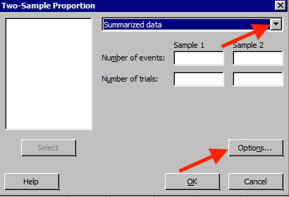
- Choose Options to display this window.
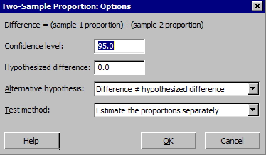
Notice how the difference is calculated. We also want to make sure that we are using the pooled estimate of the proportion as the test method. In Minitab, you need to get into options and select "Use pooled estimate of p for test." If you don't think that is reasonable to assume, then don't check the option.
You should get the following output for this example:
Test and CI for Two Proportions
| Sample | X | N | Sample p |
|---|---|---|---|
| 1 | 52 | 69 | 0.753623 |
| 2 | 120 | 131 | 0.916031 |
Difference = p (1) - p (2)
Estimate for difference: -0.162407
95% CI for difference: (-0.274625, -0.0501900)
Test for difference = 0 (vs ≠ 0): Z = -3.15 P-Value = 0.002 (Use this!)
Fisher's exact test: P-Value = 0.003 (Ignore the Fisher's exact test. This test uses a different method to calculate a test statistic from the Z-test we have learned in this lesson.)
Ignore the Fisher's p-value! The p-value highlighted above is calculated using the methods we learned in this lesson. The Fisher's test uses a different method than what we explained in this lesson to calculate a test statistic and p-value. This method incorporates a log of the ratio of observed to expected values. It's just a different technique that is more complicated to do by-hand. Minitab automatically includes both results in its output.
Try it! Section
In 1980, of 750 men 20-34 years old, 130 were found to be overweight. Whereas, in 1990, of 700 men, 20-34 years old, 160 were found to be overweight.
At the 5% significance level, do the data provide sufficient evidence to conclude that, for men 20-34 years old, a higher percentage were overweight in 1990 than 10 years earlier? Conduct the test using the p-value approach.
Let’s define 1990 as sample 1.
The null and alternative hypotheses are:
\(H_0\colon p_1-p_2=0\) vs \(H_a\colon p_1-p_2>0\)
\(n_1=700\), \(\hat{p}_1=\frac{160}{700}\)
\(n_2=750\), \(\hat{p}_2=\frac{130}{750}\)
\(\hat{p}^*=\dfrac{x_1+x_2}{n_1+n_2}=\dfrac{160+130}{700+750}=\dfrac{290}{1450}=0.2\)
The conditions are all satisfied: \(n_1\hat{p}_1\), \(n_1(1-\hat{p}_1)\), \(n_2\hat{p}_2\), and \(n_2(1-\hat{p}_2)\) are all greater than 5.
The test statistic:
\(z^*=\dfrac{\hat{p}_1-\hat{p}_2-0}{\sqrt{\hat{p}^*(1-\hat{p}^*)\left(\frac{1}{n_1}+\frac{1}{n_2}\right)}}=\dfrac{\dfrac{160}{700}-\dfrac{130}{750}}{\sqrt{0.2(1-0.2)\left(\frac{1}{700}+\frac{1}{750}\right)}}=2.6277\)
The p-value of the test based on the right-tailed alternative is:
\(\text{p-value}=P(Z>2.6277)=0.0043\)
Since our p-value of 0.0043 is less than our significance level of 5%, we reject the null hypothesis. There is enough evidence to suggest that the proportion of males overweight in 1990 is greater than the proportion in 1980.
Using Minitab
To conduct inference for two proportions with independent samples in Minitab...
- Choose Stat > Basic Statistics > 2 proportions
- Choose Options
-
Select "Difference > hypothesized difference" for 'Alternative Hypothesis.
You should get the following output.
Test and CI for Two Proportions
| Sample | X | N | Sample p |
|---|---|---|---|
| 1 | 160 | 700 | 0.228571 |
| 2 | 130 | 750 | 0.173333 |
Difference = p (1) - p (2)
Estimate for difference: 0.0552381
95% upper bound for difference: 0.0206200
Test for difference = 0 (vs < 0): Z = 2.62 P-Value = 0.004
Fisher's exact test: P-Value = 0.005 (Ignore the Fisher's exact test)