
If our test of the null hypothesis is rejected, we conclude that not all the means are equal: that is, at least one mean is different from the other means. The ANOVA test itself provides only statistical evidence of a difference, but not any statistical evidence as to which mean or means are statistically different.
For instance, using the previous example for tar content, if the ANOVA test results in a significant difference in average tar content between the cigarette brands, a follow up analysis would be needed to determine which brand mean or means differ in tar content. Plus we would want to know if one brand or multiple brands were better/worse than another brand in average tar content. To complete this analysis we use a method called multiple comparisons.
Multiple comparisons conducts an analysis of all possible pairwise means. For example, with three brands of cigarettes, A, B, and C, if the ANOVA test was significant, then multiple comparison methods would compare the three possible pairwise comparisons:
- Brand A to Brand B
- Brand A to Brand C
- Brand B to Brand C
These are essentially tests of two means similar to what we learned previously in our lesson for comparing two means. However, the methods here use an adjustment to account for the number of comparisons taking place. Minitab provides three adjustment choices. We will use the Tukey adjustment which is an adjustment on the t-multiplier based on the number of comparisons.
Note! We don’t go in the theory behind the Tukey method. Just note that we only use a multiple comparison technique in ANOVA when we have a significant result.
In the next section, we present an example to walk through the ANOVA results.
Minitab®
Using Minitab to Perform One-Way ANOVA Section
If the data entered in Minitab are in different columns, then in Minitab we use:
- Stat > ANOVA > One-Way
- Select the format structure of the data in the worksheet.
- If the responses are in one column and the factors are in their own column, then select the drop down of 'Response data are in one column for all factor levels.'
- If the responses are in their own column for each factor level, then select 'Response data are in a separate column for each factor level.'
- Next, in case we have a significant ANOVA result, and we want to conduct a multiple comparison analysis, we preemptively click 'Comparisons', the box for Tukey, and verify that the boxes for 'Interval plot for differences of means' and 'Grouping Information' are also checked.
- Click OK and OK again.
Example: Tar Content (ANOVA) Section
Test the hypothesis that the means are the same vs. at least one is different for both labs. Compare the two labs and comment.
Lab Precise
We are testing the following hypotheses:
\(H_0\colon \mu_1=\mu_2=\mu_3\) vs \(H_a\colon\text{ at least one mean is different}\)
The assumptions were discussed in the previous example.
The following is the output for one-way ANOVA for Lab Precise:
One-way ANOVA: Precise A, Precise B, Precise C
Method
| Null Hypothesis | All means are equal |
|---|---|
| Alternative Hypothesis | Not all means are equal |
| Significance Level | \(\alpha\)= 0.05 |
Equal variances were assumed for the analysis.
Factor Information
| Factor | Levels | Values |
|---|---|---|
|
Factor |
3 | Precise A, Precise B, Precise C |
Analysis of Variance
| Source | DF | Adj SS | Adj MS | F-Value | P-Value |
|---|---|---|---|---|---|
|
Factor |
2 | 12.000 | 6.00000 | 65.46 | 0.000 |
| Error | 15 | 1.375 | 0.09165 | ||
| Total | 17 | 13.375 |
Model Summary
| S | R-sq | R-sq(adj) | R-sq(pred) |
|---|---|---|---|
| 0.302743 | 89.72% | 88.35% | 85.20% |
The p-value for this test is less than 0.0001. At any reasonable significance level, we would reject the null hypothesis and conclude there is enough evidence in the data to suggest at least one mean tar content is different.
But which ones are different? The next step is to examine the multiple comparisons. Minitab provides the following output:
Means
| Factor | N | Mean | StDev | 95% CI |
|---|---|---|---|---|
| Precise A | 6 | 10.000 | 0.257 | (9.737, 10.263) |
| Precise B | 6 | 11.000 | 0.365 | (10.737, 11.263) |
| Precise C | 6 | 12.000 | 0.276 | (11.737, 12.263) |
Pooled StDev = 0.302743
Tukey Pairwise Comparisons
Grouping Information Using the Tukey Method and 95% Confidence
| Factor | N | Mean | Grouping |
|---|---|---|---|
| Precise C | 6 | 12.000 | A |
| Precise B | 6 | 11.000 | B |
| Precise A | 6 | 10.000 | C |
Means that do not share a letter are significantly different.
The Tukey pairwise comparisons suggest that all the means are different. Therefore, Brand C has the highest tar content and Brand A has the lowest.
Lab Sloppy
We are testing the same hypotheses for Lab Sloppy as Lab Precise, and the assumptions were checked. The ANOVA output for Lab Sloppy is:
One-way ANOVA: Sloppy A, Sloppy B, Sloppy C
Method
| Null Hypothesis | All means are equal |
|---|---|
| Alternative Hypothesis | Not all means are equal |
| Significance Level | \(\alpha\)= 0.05 |
Equal variances were assumed for the analysis.
Factor Information
| Factor | Levels | Values |
|---|---|---|
|
Factor |
3 |
Sloppy A, Sloppy B, Sloppy C |
Analysis of Variance
| Source | DF | Adj SS | Adj MS | F-Value | P-Value |
|---|---|---|---|---|---|
|
Factor |
2 | 12.00 | 6.000 | 1.96 | 0.176 |
| Error | 15 | 45.98 | 3.065 | ||
| Total | 17 | 57.98 |
Model Summary
| S | R-sq | R-sq(adj) | R-sq(pred) |
|---|---|---|---|
| 1.75073 | 20.70% | 10.12% | 0.00% |
Comparison
The one-way ANOVA showed statistically significant results for Lab Precise but not for Lab Sloppy. Recall that ANOVA compares the within variation and the between variation. For Lab Precise, the within variation was small compared to the between variation. This resulted in a large F-statistic (65.46) and thus a small p-value. For Lab Sloppy, this ratio was small (1.96), resulting in a large p-value.
Try it! Section
20 young pigs are assigned at random among 4 experimental groups. Each group is fed a different diet. (This design is a completely randomized design.) The data are the pig's weight, in kilograms, after being raised on these diets for 10 months (pig_weights.txt). We wish to determine whether the mean pig weights are the same for all 4 diets.
First, we set up our hypothesis test:
\(H_0\colon \mu_1=\mu_2=\mu_3=\mu_4\)
\(H_a\colon \text { at least one mean weight is different}\)
Here are the data that were obtained from the four experimental groups, as well as, their summary statistics:
| Feed 1 | Feed 2 | Feed 3 | Feed 4 |
|---|---|---|---|
| 60.8 | 68.3 | 102.6 | 87.9 |
| 57.1 | 67.7 | 102.2 | 84.7 |
| 65.0 | 74.0 | 100.5 | 83.2 |
| 58.7 | 66.3 | 97.5 | 85.8 |
| 61.8 | 69.9 | 98.9 | 90.3 |
Output from Minitab:
Descriptive Statistics: Feed 1, Feed 2, Feed 3, Feed 4
Statistics
| Variable |
N |
N* | Mean | StDev | Minimum | Maximum |
|---|---|---|---|---|---|---|
|
Feed 1 |
5 | 0 | 60.68 | 3.03 | 57.10 | 65.00 |
|
Feed 2 |
5 | 0 | 69.24 | 2.96 | 66.30 | 74.00 |
| Feed 3 | 5 | 0 | 100.34 | 2.16 | 97.50 | 102.60 |
| Feed 4 | 5 | 0 | 86.38 | 2.78 | 83.20 | 90.30 |
The smallest standard deviation is 2.16, and the largest is 3.03. Since the rule of thumb is satisfied here, we can say the equal variance assumption is not violated. The description suggests that the samples are independent. There is nothing in the description to suggest the weights come from a normal distribution. The normal probability plots are:
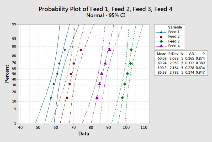
There are no obvious violations from the normal assumption, but we should proceed with caution as the sample sizes are very small.
The ANOVA output is:
One-way ANOVA: Feed 1, Feed 2, Feed 3, Feed 4
Method
| Null Hypothesis | All means are equal |
|---|---|
| Alternative Hypothesis | Not all means are equal |
| Significance Level | \(\alpha\)= 0.05 |
Equal variances were assumed for the analysis.
Factor Information
| Factor | Levels | Values |
|---|---|---|
|
Factor |
4 | Feed 1, Feed 2, Feed 3, Feed 4 |
Analysis of Variance
| Source | DF | Adj SS | Adj MS | F-Value | P-Value |
|---|---|---|---|---|---|
|
Factor |
3 | 4703.2 | 1567.73 | 206.72 | 0.000 |
| Error | 16 | 121.3 | 7.58 | ||
| Total | 19 | 4824.5 |
Model Summary
| S | R-sq | R-sq(adj) | R-sq(pred) |
|---|---|---|---|
| 2.75386 | 97.48% | 97.01% | 96.07% |
The p-value for the test is less than 0.001. With a significance level of 5%, we reject the null hypothesis. The data provide sufficient evidence to conclude that the mean weights of pigs from the four feeds are not all the same.
With a rejection of the null hypothesis leading us to conclude that not all the means are equal (i.e., at least the mean pig weight or one diet differs from the mean pig weight from the other diets) some follow up questions are:
- "Which diet type results in different average pig weights?", and
- "Is there one particular diet type that produces the largest/smallest mean weight?"
To answer these questions we analyze the multiple comparison output (the grouping information) and the interval graph.
Means
| Factor | N | Mean | StDev | 95% CI |
|---|---|---|---|---|
| Feed 1 | 5 | 60.68 | 3.03 | (58.07, 63.29) |
| Feed 2 | 5 | 69.24 | 2.96 | (66.63, 71.85) |
| Feed 3 | 5 | 100.340 | 2.164 | (97.729, 102.951) |
| Feed 4 | 5 | 86.38 | 2.78 | (83.77, 88.99) |
Pooled StDev = 2.75386
Tukey Pairwise Comparisons
Grouping Information Using the Tukey Method and 95% Confidence
| Factor | N | Mean | Grouping | ||||
|---|---|---|---|---|---|---|---|
| Feed 3 | 5 | 100.340 | A | ||||
| Feed 4 | 5 | 86.38 | B | ||||
| Feed 2 | 5 | 69.24 | C | ||||
| Feed 1 | 5 | 60.68 | D | ||||
Means that do not share a letter are significantly different.
Each of these factor levels are associated with a grouping letter. If any factor levels have the same letter, then the multiple comparison method did not determine a significant difference between the mean response. For any factor level that does not share a letter, a significant mean difference was identified. From the lettering we see each Diet Type has a different letter, i.e. no two groups share a letter. Therefore, we can conclude that all four diets resulted in statistically significant different mean pig weights. Furthermore, with the order of the means also provided from highest to lowest, we can say that Feed 3 resulted in the highest mean weight followed by Feed 4, then Feed 2, then Feed 1. This grouping result is supported by the graph of the intervals.
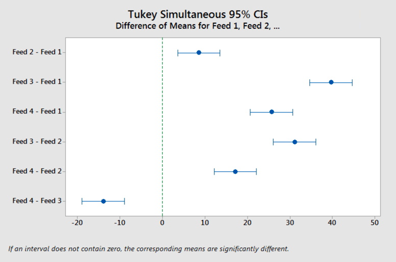
In analyzing the intervals, we reflect back on our lesson in comparing two means: if an interval contained zero, we could not conclude a difference between the two means; if the interval did not contain zero, then a difference between the two means was supported. With four factor levels, there are six possible pairwise comparisons. (Remember the binomial formula where we had the counter for the number of possible outcomes? In this case \(4\choose 2\) = 6). In inspecting each of these six intervals, we find that all six do NOT include zero. Therefore, there is a statistical difference between all four group means; the four types of diet resulted in significantly different mean pig weights.