
In this section, we present an example and review what we have covered so far in the context of the example.
Example 9-5: Student height and weight (SLR) Section
We will continue with our height and weight example. Answer the following questions.
- Is height a significant linear predictor of weight? Conduct the test at a significance level of 5%. State the regression equation.
- Does \(\beta_0\) have a meaningful interpretation?
- Find the confidence interval for the population slope and interpret it in the context of the problem.
- If a student is 70 inches, what weight could we expect?
- What is the estimated standard deviation of the error?
The model for this problem is:
\(\text{weight}=\beta_0+\beta_1\text{height}+\epsilon\)
The hypotheses we are testing are:
\(H_0\colon \beta_1=0\)
\(H_a\colon \beta_1\ne 0\)
Recall that we previously examined the assumptions. Here is a summary of what we presented before:
Assumptions
Linearity: The relationship between height and weight must be linear.
The scatterplot shows that, in general, as height increases, weight increases. There does not appear to be any clear violation that the relationship is not linear.
Independence of errors: There is not a relationship between the residuals and weight.
In the residuals versus fits plot, the points seem randomly scattered, and it does not appear that there is a relationship.
Normality of errors: The residuals must be approximately normally distributed.
Most of the data points fall close to the line, but there does appear to be a slight curving. There is one data point that clearly stands out. In the histogram, we can see that, with that one observation, the shape seems slightly right-skewed.
- Equal variances: The variance of the residuals is the same for all values of \(X\).
In this plot, there does not seem to be a pattern.
All of the assumption except for the normal assumption seem valid.
Minitab output for the height and weight data:
Model Summary
S
R-sq
R-sq(adj)
R-sq(pred)
19.1108
50.57%
48.67%
44.09%
Coefficients
Team
Coef
SE Coef
T-Value
P-Value
VIF
Constant
-222.5
72.4
-3.07
0.005
height
5.49
1.06
5.16
0.000
1.00
Regression Equation
\(\hat{\text{weight}} = -222.5+5.49\text{height}\)
The regression equation is:
\(\hat{\text{weight}}=-222.5+5.49\text{height}\)
The slope is 5.49, and the intercept is -222.5. The test for the slope has a p-value of less than 0.001. Therefore, with a significance level of 5%, we can conclude that there is enough evidence to suggest that height is a significant linear predictor of weight. We should make this conclusion with caution, however, since one of our assumptions might not be valid.
- The intercept is -222.5. Therefore, when height is equal to 0, then a person’s weight is predicted to be -222.5 pounds. It is also not possible for someone to have a height of 0 inches. Therefore, the intercept does not have a valid meaning.
The confidence interval for the population slope is:
\(\hat{\beta}_1\pm t_{\alpha/2}\hat{SE}(\hat{\beta}_1)\)
The estimate for the slope is 5.49 and the standard error for the estimate (SE Coef in the output) is 1.06. There are \(n=28\) observations so the degrees of freedom are \(28-2=26\). Using Minitab, we find the t-value to be 2.056. Putting the pieces together, the interval is:
\(5.49\pm 2.056(1.06)\)
\((3.31, 7.67)\)
We are 95% confident that the population slope is between 3.31 and 7.67. In other words, we are 95% confident that, as height increases by one inch, that weight increases by between 3.31 and 7.67 pounds, on average.
Using the regression formula with a height equal to 70 inches, we get:
\(\hat{\text{weight}}=-222.5+5.49(70)=161.8\)
A student with a height of 70 inches, we would expect a weight of 162.3 pounds. If we wanted, we could have Minitab produce a confidence interval for this estimate. We will leave this out for this example.
Using the output, under the model summary:
\(s=19.1108\)
Try it! Section
The No-Lemon used car dealership in a college town records the age (in years) and price for cars it sold in the last year (cars_sold.txt). Here is a table of this data.
age | 4 | 4 | 4 | 5 | 5 | 6 | 7 | 7 | 8 |
|---|---|---|---|---|---|---|---|---|---|
price | 6200 | 5700 | 6800 | 5600 | 4500 | 4900 | 4600 | 4300 | 4200 |
age | 8 | 8 | 9 | 9 | 10 | 10 | 11 | 12 | 13 |
|---|---|---|---|---|---|---|---|---|---|
price | 4500 | 4000 | 3200 | 3100 | 2500 | 2100 | 2600 | 2400 | 2200 |
Using the data above, answer the following questions.
- Is age a significant negative linear predictor of price? Conduct the test at a significance level of 5%.
- Does \(\beta_0\) have a meaningful interpretation?
- Find the confidence interval for the population slope and interpret it in context of the problem.
- If a car is seven years old, what price could we expect?
- What is the estimate of the standard deviation of the errors?
The linear regression model is:
\(\text{price}=\beta_0+\beta_1\text{age}+\epsilon\)
To test whether age is a statistically significant negative linear predictor of price, we can set up the following hypotheses:.
\(H_0\colon \beta_1=0\)
\(H_a\colon \beta_1< 0\)
We need to verify that our assumptions are satisfied. Let's do this in Minitab. Remember, we have to run the linear regression analysis to check the assumptions.
Assumption 1: Linearity
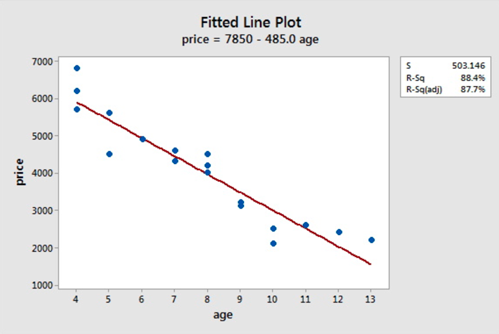
The scatterplot below shows that the relationship between age and price scores is linear. There appears to be a strong negative linear relationship and no obvious outliers.
Assumption 2: Independence of errors
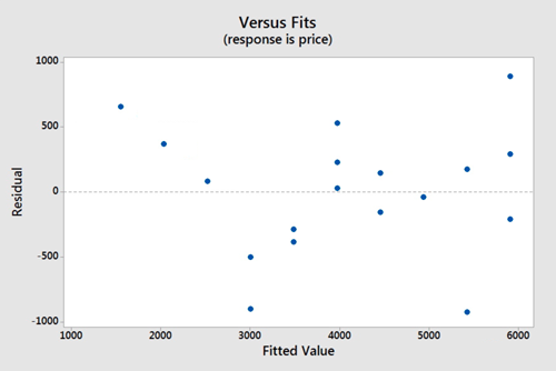
There does not appear to be a relationship between the residuals and the fitted values. Thus, this assumption seems valid.
Assumption 3: Normality of errors
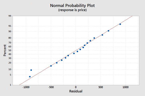
On the normal probability plot we are looking to see if our observations follow the given line. This graph does not indicate that there is a violation of the assumption that the errors are normal. If a probability plot is not an option we can refer back to one of our first lessons on graphing quantitative data and use a histogram or boxplot to examine if the residuals appear to follow a bell shape.
Assumption 4: Equal Variances

Again we will use the plot of residuals versus fits. Now we are checking that the variance of the residuals is consistent across all fitted values. This assumption seems valid.
Model Summary
S | R-sq | R-sq(adj) | R-sq(pred) |
|---|---|---|---|
503.146 | 88.39% | 87.67% | 84.41% |
Coefficients
Team | Coef | SE Coef | T-Value | P-Value | VIF |
|---|---|---|---|---|---|
Constant | 7850 | 362 | 21.70 | 0.000 | |
age | -485.0 | 43.9 | -11.04 | 0.000 | 1.00 |
Regression Equation
\(\hat{\text{price}} = 7850 - 485.0 \text{age}\)
From the output above we can see that the p-value of the coefficient of age is 0.000 which is less than 0.001. The Minitab output is for a two-tailed test and we are dealing with a left-tailed test. Therefore, the p-value for the left-tailed test is less than \(\frac{0.001}{2}\) or less than 0.0005.
We can thus conclude that age (in years) is a statistically significant negative linear predictor of price for any reasonable \(\alpha\) value.
The 95% confidence interval for the population slope is:
\(\hat{\beta}_1\pm t_{\alpha/2}\text{SE}(\hat{\beta}_1)\)
Using the output, \(\hat{\beta}_1=-485\) and the \(\text{SE}(\hat{\beta}_1)=43.9\). We need to have \(t_{\alpha/2}\) with \(n-2\) degrees of freedom. In this case, there are 18 observations so the degrees of freedom are \(18-2=16\). Using software, we find \(t_{\alpha/2}=2.12\).
The 95% confidence interval is:
\(-485\pm 2.12(43.9)\)
\((-578.068, -391.932)\)
We are 95% confident that the population slope for the regression model is between -578.068 and -391.932. In other words, we are 95% confident that, for every one year increase in age, the price of a vehicle will decrease between 391.932 and 578.068 dollars.
We can use the regression equation with \(\text{age}=7\):
\(\hat{\text{price}}=7850-485(7)=4455\)
We can expect the price to be $4455.
The residual standard error is estimated by s, which is calculated as:
\(s=\sqrt{\text{MSE}}=\sqrt{253156}=503.146\)
It is also shown as \(s\) under the model summary in the output.