
About this Course
Welcome to the course notes for STAT 415: Introduction to Mathematical Statistics. These notes are designed and developed by Penn State's Department of Statistics and offered as open educational resources. These notes are free to use under Creative Commons license CC BY-NC 4.0.
This course is part of the Online Master of Applied Statistics program offered by Penn State's World Campus.
Currently enrolled?
If you are a current student in this course, please see Canvas for your syllabus, assignments, lesson videos and communication from your instructor.
How to enroll?
If you would like to enroll and experience the entire course for credit please see 'How to enroll in a course' on the World Campus website.
Course Introduction Section
We spent all of our time in Stat 414 filling up a probability toolbox just so we'd be in a position in Stat 415 to fill up a statistics toolbox that we can use to answer research questions. For example, suppose someone (a researcher? pollster? student?) is interested in learning something (average blood pressure? purchasing habits? median age?) about a population of somebodies (the elderly? students? trees?). Someone might even be interested in comparing two or more populations (males vs. females? athletes vs. non-athletes? oaks vs. elms?). Unfortunately, populations are often too large to measure all of the somebodies. So, we take a random sample of some bodies from the population. We then use the measurements (data) taken on the sample to draw conclusions about the larger population. We use probability calculations, such as those learned in Stat 414, to help draw the conclusions.
Example #1 
A researcher is interested in answering the following research question: What proportion of American internet users are addicted to the internet? The researcher deems that a person is addicted to the internet if the person exhibits at least five of ten possible characteristics, such as using the internet to escape from his/her problems, trying unsuccessfully to cut back his/her usage, and finding himself/herself preoccupied with the internet when no longer sitting at a computer.
What proportion of the 230,630,000 American internet users (Source: World Bank, 2008) are addicted to the internet?
Answer
We aren't going to answer the researcher's question, but rather pretend we will (much like my five-year-old daughter loves to pretend)! The researcher can't evaluate the behavior of all of the 230-some million American internet users. Instead, suppose the researcher takes a random sample of 17,251 American internet users and evaluates them for internet addiction. The resulting data would be a bunch ...17,251 data points, to be exact... of yeses and nos:
yes yes no yes no no no no no no ...
The data in such a raw format are not particularly helpful, so the researcher uses a "sample statistic" to summarize the data. Based on his sample, the researcher calculates the proportion in his sample that he deemed addicted to the internet:
\(\hat{p}=\dfrac{990}{17521}=0.057\)
That \(p\) with a caret (^) over it is, by the way, and perhaps not surprisingly, called "p-hat." It, in general, denotes the proportion in a sample with a particular characteristic.
Now, that sample proportion of 0.057 is all well and good. But, we aren't interested in the proportion in the sample who are addicted to the internet. We are interested in knowing the "population parameter," that is, \(p\), the true, unknown, proportion of the population who are addicted to the internet.
We'll soon learn, in Section 6 specifically, that we can use a confidence interval to help quantify the value of a population parameter. A "confidence interval" is a range or interval of values that we can be confident contains the population parameter of interest, in this case, \(p\), the true unknown population proportion. When all is said and done, by calculating a confidence interval for \(p\), the researcher should be able to make a statement such as this:
"We can be 95% confident that the true proportion of Americans addicted to the internet is between 0.0534 and 0.0606 (0.057±0.0036)."
By the way, the interval is so narrow here, because the sample size is so large. Polling sample sizes are typically in the range of 1000 to 1600 respondents.
Section 1
The previous example illustrates the kind of question we'll answer in the lessons in Section 6 (and one lesson in Section 10). Specifically, the lessons in Section 6 (and one of the lessons in Section 10) focus on deriving good "point estimates" and "confidence intervals" for:
| Population parameter...based on... | Sample statistic |
|---|---|
| population mean, \(\mu\) | sample mean, \(\bar{x}\) |
| difference in two population means, \(\mu_1-\mu_2\) | difference in sample means, \(\bar{x}_1-\bar{x}_2\) |
| population variance, \(\sigma^2\) | sample variance, \(s^2\) |
| population proportion, \(p\) | sample proportion, \(\hat{p}\) |
| difference in two population proportions, \(p_1-p_2\) | difference in sample proportions, \(\hat{p}_1-\hat{p}_2\) |
In these lessons, we'll work on not only obtaining formulas for the estimates and intervals but also on arguing that they are "good" in some way... unbiased, for example. We'll also address practical matters, such as how sample size affects the length of our derived confidence intervals. And, we'll also work on deriving good point estimates and confidence intervals for a least-squares regression line through a set of \((x,y)\) data points.
 Example #2
Researchers are interested in answering the following research question: Does eating nuts regularly lower the risk of heart attacks in women? The researchers deem that a woman eats nuts regularly if she eats more than five ounces of nuts in one week.
Does eating nuts regularly lower the risk of heart attacks in women?
Answer
We'll attempt to answer the researchers' question using data collected on a sample of 86,000 American women nurses in the national Nurses Health Study. In this case, the population of interest is all American women, but based on the sample used, it is technically more correct to say that the population is all American women nurses. We can divide the sample of 86,000 women into three groups... those who eat more than five ounces of nuts weekly, those who eat some but less than five ounces of nuts weekly, and those who eat no nuts weekly. Doing so, we obtain a division of the sample:
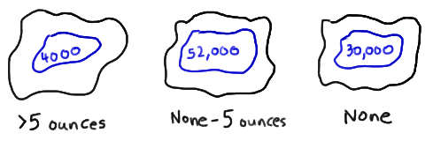
That is, 4000 women in the sample eat more than five ounces of nuts weekly, 52000 women who eat some but less than five ounces of nuts weekly, and 30000 who eat no nuts weekly. Of the 4000 women who eat more than five ounces of nuts weekly, 44 suffered a heart attack. Of the 52000 women who eat some but less than five ounces of nuts weekly, 669 suffered heart attacks. And, of the 30000 women who don't eat nuts at all, 554 suffered a heart attack. Using these data, we can calculate the sample proportion in each group who suffered a heart attack. Doing so, we obtain:
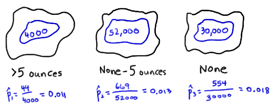
We'll soon learn, in Section 7, that using these sample statistics, we can conduct what is called a "hypothesis test" to help answer the research question. If nuts have no impact on the population, the difference in the population proportions is 0, that is \(p_3-p_1=0\). But note that the difference in the sample proportions is not 0:
\(\hat{p}_3-\hat{p}_1=0.018-0.011=0.007\)
The question we need to answer is:
"How likely is it (that is, what is the probability) that the difference in the sample proportions would be as large as 0.007 if the difference in population proportions is 0?"
If the answer to the question is "not likely" (that is, the probability is close to 0), then we would conclude that the population proportions differ. That is, we would conclude that evidence is strong that eating nuts regularly lowers the risk of heart attacks in women.
Section 2
The previous example illustrates the kind of question we'll answer in the lessons in Section 7 (and three lessons in Section 10). Specifically, the lessons in Section 7 (and three of the lessons in Section 10) focus on deriving good "hypothesis tests" for the same population parameters addressed in Section 6:
| Population parameter...based on... | Sample statistic |
|---|---|
| population mean, \(\mu\) | sample mean, \(\bar{x}\) |
| difference in two population means, \(\mu_1-\mu_2\) | difference in sample means, \(\bar{x}_1-\bar{x}_2\) |
| population variance, \(\sigma^2\) | sample variance, \(s^2\) |
| population proportion, \(p\) | sample proportion, \(\hat{p}\) |
| difference in two population proportions, \(p_1-p_2\) | difference in sample proportions, \(\hat{p}_1-\hat{p}_2\) |
In these lessons, we'll work on not only obtaining formulas for the hypothesis tests but also on arguing that they are "good" in some way... powerful, for example. We'll also learn how to use the analysis of variance technique to compare more than two means, as well as how to use a set of \(x,y\) data points to test for a linear relationship between the \(x\)-variable and \(y\)-variable.
 Example #3
A biologist who studies spiders selected a random sample of 20 spiders and measured the lengths (in millimeters) of one of the front legs of the 20 spiders. What is the median length of the front legs of all such spiders in the population?
Answer
Again, we cannot possibly measure the length of the front legs of all of the spiders in the population. We can take a random sample of spiders from the population though and measure their front legs. The biologist did this for us by obtaining:
15.10 13.55 15.75 20.00 15.45 13.60 16.45 14.05 16.95 19.05
16.40 17.05 15.25 16.65 16.25 17.75 15.40 16.80 17.55 19.05
It doesn't take much work to determine that the median front leg length of this sample of 20 spiders is 16.425 millimeters. Now again, that sample median of 16.425 is all well and good. But, we aren't interested in the median of the sample. We are interested in knowing the median of the population.
It seems reasonable to think that we could apply the methods of Section 6 here. That is, we could find a confidence interval for the population median. The only problem is that the material in Section 6 doesn't address confidence intervals for a median. Why's that? Well, that's because the confidence intervals in Section 6 are derived by making assumptions about the distribution of the data, assuming that the front leg length of spiders is normally distributed, for example.
We'll soon learn that the methods in Section 8, called nonparametric methods, are derived without making assumptions about the distribution of the underlying data. After we have worked our way through Section 8, we'll be able to make this kind of statement for the biologist of this example:
"We can be 95% confident that median length of the front legs of all spiders is between 15.40 and 17.05 millimeters.
And, we will be able to make that statement without making any assumptions about the distribution of the front leg length of spiders.
Section 3
The previous example illustrates the kind of question we'll answer in the lessons in Section 8. Specifically, we'll learn:
- how to use a chi-square goodness-of-fit test to assess whether a set of data follow a particular probability distribution
- how to use a chi-square test to test for the independence between two categorical variables (gender and opinion, for example)
- how to use order statistics to determine sample percentiles and confidence intervals for the corresponding population percentiles
- how to use a Wilcoxon test to compare the medians of two populations
- how to use a run test to test for the randomness of measurements
- how to use the Kolmogorov-Smirnov goodness-of-fit test to assess whether a set of data follow a particular probability distribution
- how to resample data as a way of learning the distribution of a sample statistic
Again, all of the methods we learn in Section 8 are developed making little or no assumptions about the distribution of the underlying data.
 Example #4
The following amounts are bet on horses A, B, and C to win:
- Horse A: \$400,000
- Horse B: \$250,000
- Horse C: \$350,000
Suppose the track wants to take 10%, or \$100,000 off the top. How much should the track pay a bettor for winning with a \$2 bet on Horse A?
Answer
We'll soon learn, in Section 9, how Bayesian statisticians use subjective probability to answer this kind of question. In short, we can use the amount bet on horse A as an indicator of the bettors' feelings about which horse is going to win. That is, the probability that horse A will win is:
\(\dfrac{400000}{1000000}=0.40\)
Therefore, the odds against horse A winning is:
\(\dfrac{1-0.40}{0.40}=1.5\)
So, for a \$1 bet on horse A, the track could pay a bettor \$1.50; and for a \$2 bet, the track could pay \$3.00. We can't stop our calculation there, though, as the track wants to skim some money...10%, to be exact... off of the top. So, rather than paying \$3.00 on a \$2.00 bet, the track should pay \$3.00−0.10(3) = \$2.70.
Section 4
In addition to learning how to make the kind of calculation illustrated in the above example, we'll learn how Bayesians estimate the value of a population parameter, such as a mean or variance parameter.
That does it! That's the summary in a nutshell of where we'll be going in this Stat 415 course. Now, let's pick up our probability toolbox, jump right in and get to work!