Our work so far Section
So far, we have shown that the formula:
\(\bar{x}\pm z_{\alpha/2}\left(\dfrac{\sigma}{\sqrt{n}}\right)\)
is appropriate for finding a confidence interval for a population mean if two conditions are met:
- The population standard deviation \(\sigma\) is known, and
- \(X_1, X_2, \ldots, X_n\) are normally distributed. (The truth is that \(X_1, X_2, \ldots, X_n\) need not be normally distributed as long as the sample size \(n\) is large enough for the Central Limit Theorem to apply. In this case, the confidence interval is an approximate confidence interval.)
Now, as suggested earlier in this lesson, it is unrealistic to think that we'd ever be in a situation where the first condition would be met. That is, when would we ever know the population standard deviation \(\sigma\), but not the population mean \(\mu\)? Let's entertain, then, the realistic situation in which not only the population mean \(\mu\) is unknown, but also the population standard deviation \(\sigma\) is unknown.
What if \(\sigma\) is unknown? Section
Yes, the reasonable thing to do is to estimate the population standard deviation \(\sigma\) with the sample standard deviation:
\(S=\sqrt{\dfrac{1}{n-1}\sum\limits_{i=1}^n (X_i-\bar{X})^2}\)
Then, in deriving the confidence interval, we'd start out with:
\(\dfrac{\bar{X}-\mu}{S/\sqrt{n}}\)
instead of:
\(\dfrac{\bar{X}-\mu}{\sigma/\sqrt{n}}\sim N(0,1)\)
Then, to derive the confidence interval, in this case, we just need to know how:
\(T=\dfrac{\bar{X}-\mu}{S/\sqrt{n}}\)
is distributed!
How is \(T=\dfrac{\bar{X}-\mu}{S/\sqrt{n}}\) distributed? Section
Given that the ratio is typically denoted by the capital letter \(T\), we probably shouldn't be surprised that the ratio follows a \(T\) distribution!
If \(X_1, X_2, \ldots, X_n\) are normally distributed with mean \(\mu\) and variance \(\sigma^2\), then:
\(T=\dfrac{\bar{X}-\mu}{S/\sqrt{n}}\)
follows a \(T\) distribution with \(n-1\) degrees of freedom.
Proof
The proof is as simple as recalling a few distributional results from our work in Stat 414. Recall the definition of a \(T\) random variable, namely if \(Z\sim N(0,1)\) and \(U\sim \chi^2_{(r)}\) are independent, then:
\(T=\dfrac{Z}{\sqrt{U/r}}\)
follows the \(T\) distribution with \(r\) degrees of freedom. Furthermore, recall that if \(X_1, X_2, \ldots, X_n\) are normally distributed with mean \(\mu\) and variance \(\sigma^2\), then:
-
\(Z=\dfrac{\bar{X}-\mu}{\sigma/\sqrt{n}}\sim N(0,1)\)
-
\(\dfrac{(n-1)S^2}{\sigma^2}\sim \chi^2_{n-1}\)
-
\(\bar{X}\) and \(S^2\) are independent
Now, we just have to put all that we've remembered together:
\(T=\dfrac{ \frac{\bar{x}-\mu}{\sigma/\sqrt{n}} }{\sqrt{\frac{\frac{(n-1)s^2}{\sigma^2}}{n-1}}}=\dfrac{\bar{x}-\mu}{\sigma/\sqrt{n}}\left(\frac{\sigma}{s}\right)=\dfrac{\bar{x}-\mu}{s/\sqrt{n}}\sim t_{n-1}\)
The first equality simply defines a \(T\) random variable using the first, second, and third bullet point above. The second equality comes from canceling out the \(n-1\) terms in the denominator. The third equality comes from canceling out the \(\sigma\) terms, leaving us with:
\(T=\dfrac{\bar{X}-\mu}{S/\sqrt{n}}\)
following a \(T\) distribution with \(n-1\) degrees of freedom, as was to be proved!
Now that we have the distribution of \(T=\dfrac{\bar{X}-\mu}{S/\sqrt{n}}\) behind us, we can derive the confidence interval for a population mean in the realistic situation that \(\sigma\) is unknown.
If \(X_1, X_2, \ldots, X_n\) are normally distributed random variables with mean \(\mu\) and variance \(\sigma^2\), then a \((1-\alpha)100\%\) confidence interval for the population mean \(\mu\) is:
\(\bar{x}\pm t_{\alpha/2,n-1}\left(\dfrac{s}{\sqrt{n}}\right)\)
This interval is often referred to as the "\(t\)-interval for the mean."
Proof
The proof is very similar to that for the \(Z\)-interval for the mean. We start by drawing a picture of a \(T\)-distribution with \(n-1\) degrees of freedom:
From the diagram, we can see that the following probability statement is true:
\(P[-t_{\alpha/2,n-1}\leq T \leq t_{\alpha/2,n-1}]=1-\alpha \)
Then, simply replacing \(T\), we get:
\(P\left[-t_{\alpha/2,n-1}\leq \dfrac{\bar{X}-\mu}{s/\sqrt{n}} \leq t_{\alpha/2,n-1}\right]=1-\alpha \)
Let's again focus only on the inequality inside the brackets for a bit. Because we manipulate each of the three sides of the inequality equally, each of the following statements are equivalent:
\begin{array}{rccl} -t_{\alpha/2,n-1} & \leq & \dfrac{\bar{X}-\mu}{s/\sqrt{n}} & \leq & t_{\alpha/2,n-1}\\ -t_{\alpha/2,n-1}\left(\dfrac{s}{\sqrt{n}}\right) & \leq & \bar{X}-\mu & \leq & +t_{\alpha/2,n-1}\left(\dfrac{s}{\sqrt{n}}\right)\\ -\bar{X}-t_{\alpha/2,n-1}\left(\dfrac{s}{\sqrt{n}}\right) & \leq & -\mu & \leq & -\bar{X}+t_{\alpha/2,n-1}\left(\dfrac{s}{\sqrt{n}}\right)\\ \bar{X}-t_{\alpha/2,n-1}\left(\dfrac{s}{\sqrt{n}}\right) & \leq & \mu &\leq & \bar{X}+t_{\alpha/2,n-1}\left(\dfrac{s}{\sqrt{n}}\right) \end{array}
That is, we have shown that a \((1-\alpha)100\%\) confidence interval for the mean \(\mu\) is:
\(\left[\bar{X}-t_{\alpha/2,n-1}\left(\dfrac{s}{\sqrt{n}}\right),\bar{X}+t_{\alpha/2,n-1}\left(\dfrac{s}{\sqrt{n}}\right)\right]\)
as was to be proved.
Just one more thing. Before we go off and work through an example, let's clarify a bit of confidence interval terminology.
- \(t\)-interval
-
With the formula for the \(t\)-interval:
\(\bar{x}\pm t_{\alpha/2,n-1}\left(\dfrac{s}{\sqrt{n}}\right)\)
in mind, we say that:
- \(\bar{x}\) is a "point estimate" of \(\mu\)
- \(\bar{x}\pm t_{\alpha/2,n-1}\left(\dfrac{s}{\sqrt{n}}\right)\) is an "interval estimate" of \(\mu\)
- \(\dfrac{s}{\sqrt{n}}\) is the "standard error of the mean"
- \(t_{\alpha/2,n-1}\left(\dfrac{s}{\sqrt{n}}\right)\) is the "margin of error"
Now, let's take a look at an example!
Example 2-2 Section

A random sample of 16 Americans yielded the following data on the number of pounds of beef consumed per year:
118 115 125 110 112 130 117 112 115 120 113 118 119 122 123 126
What is the average number of pounds of beef consumed each year per person in the United States?
Answer
To help answer the question, we'll calculate a 95% confidence interval for the mean. As the above theorem states, in order for the \(t\)-interval for the mean to be appropriate, the data must follow a normal distribution. We can use a normal probability plot to provide evidence that the data are (sufficiently) normally distributed:
That is, because the data points fall at least approximately on a straight line, there's no reason to conclude that the data are not normally distributed. That's convoluted statistician talk for "we're good to go." Now, punching the \(n=16\) data points into a calculator (or statistical software), we can easily determine that the sample mean is 118.44 and the sample standard deviation is 5.66. For a 95% confidence interval with \(n=16\) data points, we need:
\(t_{0.025,15}=2.1314\)
Now, we have all of the necessary elements to calculate the 95% confidence interval for the mean. It is:
\(\bar{x}\pm t_{0.025,15}\left(\dfrac{s}{\sqrt{n}}\right)=118.44\pm 2.1314\left(\dfrac{5.66}{\sqrt{16}}\right)\)
Simplifying, we get:
\(118.44\pm 3.016\)
or:
\((115.42,121.46)\)
That is, we can 95% confident that the average amount of beef consumed each year per person in the United States is between 115.42 and 121.46 pounds. Wow, that's a lot of beef!
Minitab®
Using Minitab Section
Again, statistical software, such as Minitab, can make calculating confidence intervals easier. To ask Minitab to calculate a \(t\)-interval for a mean \(\mu\), you need to do this:
-
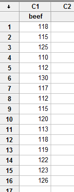
Enter the data in one of the columns. Here's the data from the above example entered in the C1 column:
-
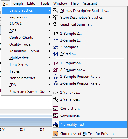
Convince yourself that the data come from a normal distribution... either from your previous experience or by creating a normal probability plot. To ask Minitab to generate a normal probability plot, under the Stat menu, select Basic Statistics, and then select Normality Test...:
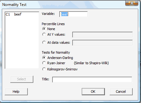
In the pop-up window that appears, select the data (column) to be plotted so that it appears in the box labeled Variable:
Select OK. When you do so, a new graphics window should appear containing the normal probability plot:
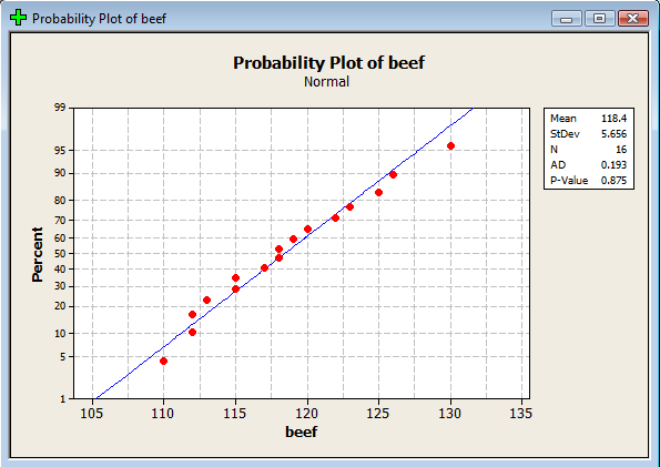
(The plot appearing in the example above was generated in Minitab using different commands. That's why it looks different from this one.)
-
Then, after convincing yourself that the normality assumption is appropriate, under the Stat menu, select Basic Statistics, and then select 1-Sample t...:
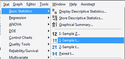
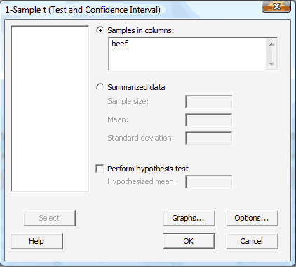
In the pop-up window that appears, select the column (data) to be analyzed so that it appears in the box labeled Samples in columns:
-
Select OK. The confidence interval output will appear in the Session window. Here is what the Minitab output looks like for the beef example:
One-Sample T: beef
| Variable | N | Mean | StDev | SE Mean | 95% CI |
|---|---|---|---|---|---|
| beef | 16 | 118.44 | 5.66 | 1.41 | (115.42, 121.45) |