Example 3-2 Section

Are there physiological indicators associated with schizophrenia? In a 1990 article, researchers reported the results of a study that controlled for genetic and socioeconomic differences by examining 15 pairs of identical twins, where one of the twins was schizophrenic and the other not. The researchers used magnetic resonance imaging to measure the volumes (in cubic centimeters) of several regions and subregions inside the twins' brains. The following data came from one of the subregions, the left hippocampus:
What is the magnitude of the difference in the volumes of the left hippocampus between (all) unaffected and affected individuals?
| Pair | Unaffect | Affect |
|---|---|---|
| 1 | 1.94 | 1.27 |
| 2 | 1.44 | 1.63 |
| 3 | 1.56 | 1.47 |
| 4 | 1.58 | 1.39 |
| 5 | 2.06 | 1.93 |
| 6 | 1.66 | 1.26 |
| 7 | 1.75 | 1.71 |
| 8 | 1.77 | 1.67 |
| 9 | 1.78 | 1.28 |
| 10 | 1.92 | 1.85 |
| 11 | 1.25 | 1.02 |
| 12 | 1.93 | 1.34 |
| 13 | 2.04 | 2.02 |
| 14 | 1.62 | 1.59 |
| 15 | 2.08 | 1.97 |
Answer
Let \(X_i\) (labeled Unaffect) denote the volume of the left hippocampus of unaffected individual \(i\), and let \(Y_i\) (labeled Affect) denote the volume of the left hippocampus of affected individual \(i\). Then, we are interested in finding a confidence interval for the difference of the means:
\(\mu_X-\mu_Y\)
If the pairs of measurements were independent, the calculation of the confidence interval would be trivial, as we could calculate either a pooled two-sample \(t\)-interval or a Welch's \(t\)-interval depending on whether or not we could assume the population variances were equal. But, alas, the \(X_i\) and \(Y_i\) measurements are not independent, since they are measured on the same pair \(i\) of twins! So we can skip that idea of using either of the intervals we've learned so far in this lesson.
Fortunately, though, the calculation of the confidence interval is still trivial! The difference in the measurements of the unaffected and affected individuals, that is:
\(D_i=X_i-Y_i\)
removes the twin effect and therefore quantifies the direct effect of schizophrenia for each (independent) pair \(i\) of twins. In that case, then, we are interested in estimating the mean difference, that is:
\(\mu_D=\mu_X-\mu_Y\)
That is, we have reduced the problem to that of a single population of measurements, which just so happen to be independent differences. Then, we're right back to the situation in which we can use the one-sample \(t\)-interval to estimate \(\mu_D\). We just have to take the extra step of calculating the differences (labeled DiffU−A):
Then, the formula for a 95% confidence interval for \(\mu_D\) is:
\(\bar{d} \pm t_{0.025,14}\left(\dfrac{s_d}{\sqrt{n}}\right)\)
Summarizing the difference data, and consulting a \(t\)-table, we get:
\(0.1987 \pm 2.1448 \left(\dfrac{0.2383}{\sqrt{15}}\right)\)
which simplifies to this:
\(0.1987 \pm 2.1448(0.0615)\)
and this:
\(0.1987 \pm 0.1319\)
and finally this:
\((0.0668,0.3306)\)
| Pair | Unaffect | Affect | DiffU-A |
|---|---|---|---|
| 1 | 1.94 | 1.27 | 0.67 |
| 2 | 1.44 | 1.63 | -0.19 |
| 3 | 1.56 | 1.47 | 0.09 |
| 4 | 1.58 | 1.39 | 0.19 |
| 5 | 2.06 | 1.93 | 0.13 |
| 6 | 1.66 | 1.26 | 0.40 |
| 7 | 1.75 | 1.71 | 0.04 |
| 8 | 1.77 | 1.67 | 0.10 |
| 9 | 1.78 | 1.28 | 0.50 |
| 10 | 1.92 | 1.85 | 0.07 |
| 11 | 1.25 | 1.02 | 0.23 |
| 12 | 1.93 | 1.34 | 0.59 |
| 13 | 2.04 | 2.02 | 0.02 |
| 14 | 1.62 | 1.59 | 0.03 |
| 15 | 2.08 | 1.97 | 0.11 |
That is, we can be 95% confident that the mean size for unaffected individuals is between 0.067 and 0.331 cubic centimeters larger than the mean size for affected individuals.
Let's summarize the method we used in deriving a confidence interval for the difference in the means of two dependent populations.
Result.
In general, when dealing with pairs of dependent measurements, we should use \(\bar{d}\), the sample mean difference, to estimate \(\mu_D\), the population mean difference. As long as the differences are normally distributed, we should use the \((1-\alpha)100\%\) \(t\)-interval for the mean, but now treating the differences as the sample data:
\(\bar{d} \pm t_{\alpha/2,n-1}\left(\dfrac{s_d}{\sqrt{n}}\right)\)
Minitab®
Using Minitab Section
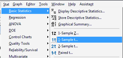
We've already learned how to use Minitab to calculate a \(t\)-interval for a mean, namely under the Stat menu, select Basic Statistics and then 1-Sample t...:

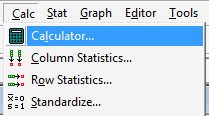
In calculating a paired t-interval, though, we have to take one additional step, namely that of calculating the differences. First, label an empty column in the worksheet that will contain the differences, DiffU-A, say. Then, under the Calc menu, select Calculator...:

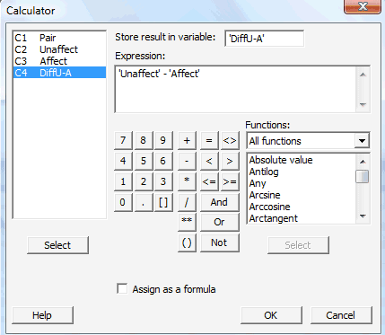
In the pop-up window that appears, click on the box labeled Store result in variable, and then in the left box containing the names of your worksheet columns, double-click on the column labeled as DiffU-A. Then, click on the box labeled Expression, and use the calculator to tell Minitab to take the differences between the relevant columns, Unaffect and Affect, here:

When you click on OK, the output will appear in the Session window, looking something like this, with the 95% confidence interval circled in red:
One-Sample T: DiffU-A
| Variable | N | Mean | StDev | SE Mean | 95.0% CI |
|---|---|---|---|---|---|
| DiffU-A | 15 | 0.1987 | 0.2383 | 0.0615 | ( 0.0667, 0.3306) |
Common Uses of the Paired t-Interval
In the previous example, measurements were taken on one person who was similar in some way with another person, using a design procedure known as matching. That is just one way in which data can be considered "paired." The most common ways in which data can be paired are:
-
A person is matched with a similar person. For example, a person is matched to another person with a similar intelligence (IQ scores, for example) to compare the effects of two educational programs on test scores.
-
Before and after studies. For example, a person is weighed, and then put on a diet, and weighed again.
-
A person serves as his or her own control. For example, a person takes an asthma drug called GoodLungs to assess the improvement on lung function, has a period of 8-weeks in which no drugs are taken (known as a washout period), and then takes a second asthma drug called EvenBetterLungs to again assess the improvement on lung function.