All of our examples thus far have involved unique observations. That is, there were no tied observations. Dealing with ties is simple enough. If the absolute values of the differences from \(m_0\) of two or more observations are equal, each observation is assigned the average of the corresponding ranks. The change this causes in the distribution of W is not all that great.
Example 20-5 Section

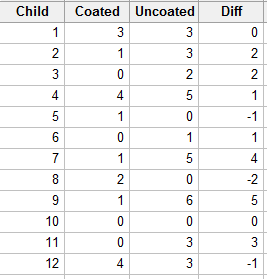
Dental researchers have developed a new material for preventing cavities, a plastic sealant that is applied to the chewing surfaces of teeth. To determine whether the sealant is effective, it was applied to half of the teeth of each of 12 school-aged children. After two years, the number of cavities in the sealant-coated teeth and in the uncoated teeth were counted, resulting in the following data:

Is there sufficient evidence to indicate that sealant-coated teeth are less prone to cavities than are untreated teeth? (From Wackerly, Mendenhall, & Scheaffer, seventh edition.)
Answer
Let X denote the number of cavities in the uncoated teeth, and Y denote the number of cavities in the coated teeth. Then, we're interested in analyzing the differences D = X−Y. Specifically, if m is the median of the differences D = X−Y, then we're interested in testing the null hypothesis \(H_0 \colon m = 0\) against the alternative hypothesis \(H_A \colon m > 0\). Analyzing the differences, we see that two of the differences are 0, and so we eliminate them from the analysis:

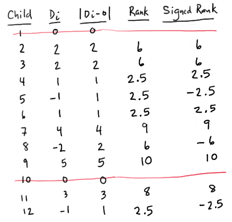
Assigning ranks to the remaining 10 data points, we see that we have two sets of tied observations. Because there are four 1s, we assign them the average of the ranks 1, 2, 3, and 4, that is, 2.5. Having used up the ranks 1, 2, 3, and 4, because 2 is the next set of tied observations, the three 2s are assigned the average of the ranks 5, 6, and 7, that is, 6. Having used up the ranks from 1 to 7, the remaining three unique observations get assigned the ranks 8, 9, and 10. When all is said and done, W, the sum of the positive ranks is:
W = 6 + 6 + 2.5 + 2.5 + 9 + 10 + 8 = 44
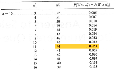
The statistical table for W:

tells us that the P-value is P(W ≥ 44) = 0.053. There is just barely not enough evidence, at the 0.05 level, to reject the null hypothesis. (I do imagine that a larger sample may have lead to a significant result.)
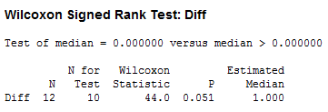
Alternatively, we could have completely ignored the condition of the data, that is, whether or not there were ties, and put the data into the black box of Minitab, getting:

We see that our analysis is consistent with the results from Minitab, namely 10 data points yield a Wilcoxon statistic of 44.0 and a P-value of 0.051 (round-off error).