Let's start right out by stating the confidence interval for one population variance.
If \(X_{1}, X_{2}, \dots , X_{n}\) are normally distributed and \(a=\chi^2_{1-\alpha/2,n-1}\) and \(b=\chi^2_{\alpha/2,n-1}\), then a \((1−\alpha)\%\) confidence interval for the population variance \(\sigma^2\) is:
\(\left(\dfrac{(n-1)s^2}{b} \leq \sigma^2 \leq \dfrac{(n-1)s^2}{a}\right)\)
And a \((1−\alpha)\%\) confidence interval for the population standard deviation \(\sigma\) is:
\(\left(\dfrac{\sqrt{(n-1)}}{\sqrt{b}}s \leq \sigma \leq \dfrac{\sqrt{(n-1)}}{\sqrt{a}}s\right)\)
Proof
We learned previously that if \(X_{1}, X_{2}, \dots , X_{n}\) are normally distributed with mean \(\mu\) and population variance \(\sigma^2\), then:
\(\dfrac{(n-1)S^2}{\sigma^2} \sim \chi^2_{n-1}\)
Then, using the following picture as a guide:
with (\(a=\chi^2_{1-\alpha/2}\)) and (\(b=\chi^2_{\alpha/2}\)), we can write the following probability statement:
\(P\left[a\leq \dfrac{(n-1)S^2}{\sigma^2} \leq b\right]=1-\alpha\)
Now, as always it's just a matter of manipulating the quantity in the parentheses. That is:
\(a\leq \dfrac{(n-1)S^2}{\sigma^2} \leq b\)
Taking the reciprocal of all three terms, and thereby changing the direction of the inequalities, we get:
\(\dfrac{1}{a}\geq \dfrac{\sigma^2}{(n-1)S^2} \geq \dfrac{1}{b}\)
Now, multiplying through by \((n−1)S^2\), and rearranging the direction of the inequalities, we get the confidence interval for \(\sigma ^2\):
\(\dfrac{(n-1)S^2}{b} \leq \sigma^2 \leq \dfrac{(n-1)S^2}{a}\)
as was to be proved. And, taking the square root, we get the confidence interval for \(\sigma\):
\(\dfrac{\sqrt{(n-1)S^2}}{\sqrt{b}} \leq \sigma \leq \dfrac{\sqrt{(n-1)S^2}}{\sqrt{a}}\)
as was to be proved.
Example 32-1 Section

A large candy manufacturer produces, packages and sells packs of candy targeted to weigh 52 grams. A quality control manager working for the company was concerned that the variation in the actual weights of the targeted 52-gram packs was larger than acceptable. That is, he was concerned that some packs weighed significantly less than 52-grams and some weighed significantly more than 52 grams. In an attempt to estimate \(\sigma\), the standard deviation of the weights of all of the 52-gram packs the manufacturer makes, he took a random sample of n = 10 packs off of the factory line. The random sample yielded a sample variance of 4.2 grams. Use the random sample to derive a 95% confidence interval for \(\sigma\).
Answer
First, we need to determine the two chi-square values with (n−1) = 9 degrees of freedom. Using the table in the back of the textbook, we see that they are:
\(a=\chi^2_{1-\alpha/2,n-1}=\chi^2_{0.975,9}=2.7\) and \(b=\chi^2_{\alpha/2,n-1}=\chi^2_{0.025,9}=19.02\)
Now, it's just a matter of substituting in what we know into the formula for the confidence interval for the population variance. Doing so, we get:
\(\left(\dfrac{9(4.2)}{19.02} \leq \sigma^2 \leq \dfrac{9(4.2)}{2.7}\right)\)
Simplifying, we get:
\((1.99\leq \sigma^2 \leq 14.0)\)
We can be 95% confident that the variance of the weights of all of the packs of candy coming off of the factory line is between 1.99 and 14.0 grams-squared. Taking the square root of the confidence limits, we get the 95% confidence interval for the population standard deviation \(\sigma\):
\((1.41\leq \sigma \leq 3.74)\)
That is, we can be 95% confident that the standard deviation of the weights of all of the packs of candy coming off of the factory line is between 1.41 and 3.74 grams.
Minitab®
Using Minitab Section
Confidence Interval for One Variance
-
Under the Stat menu, select Basic Statistics, and then select 1 Variance...:
-
In the pop-up window that appears, in the box labeled Data, select Sample variance. Then, fill in the boxes labeled Sample size and Sample variance.
-
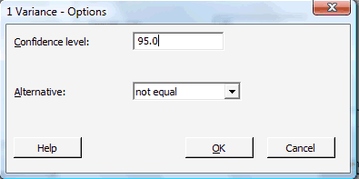
Click on the button labeled Options... In the pop-up window that appears, specify the confidence level and "not equal" for the alternative.

Then, click on OK to return to the main pop-up window.
-
Then, upon clicking OK on the main pop-up window, the output should appear in the Session window:
Test and CI for One Variance
Method
The chi-square method is only for the normal distribution.
The Bonett method cannot be calculated with summarized data.
Statistics
| N | StDev | Variance |
|---|---|---|
| 10 | 2.05 | 4.20 |
95% Confidence Intervals
| Method | CI for StDev |
CI for Variance |
|---|---|---|
| Chi-Square | (1.41, 3.74) | (1.99, 14.00) |