So far, all of our discussion has been on finding a confidence interval for the population mean \(\mu\) when the data are normally distributed. That is, the \(t\)-interval for \(\mu\) (and \(Z\)-interval, for that matter) is derived assuming that the data \(X_1, X_2, \ldots, X_n\) are normally distributed. What happens if our data are skewed, and therefore clearly not normally distributed?
Well, it is helpful to note that as the sample size \(n\) increases, the \(T\) ratio:
\(T=\dfrac{\bar{X}-\mu}{\frac{S}{\sqrt{n}}}\)
approaches an approximate normal distribution regardless of the distribution of the original data. The implication, therefore, is that the \(t\)-interval for \(\mu\):
\(\bar{x}\pm t_{\alpha/2,n-1}\left(\dfrac{s}{\sqrt{n}}\right)\)
and the \(Z\)-interval for \(\mu\):
\(\bar{x}\pm z_{\alpha/2}\left(\dfrac{s}{\sqrt{n}}\right)\)
(with the sample standard deviation s replacing the unknown population standard deviation \(\sigma\)!) yield similar results for large samples. This result suggests that we should adhere to the following guidelines in practice.
In practice! Section
-
Use \(\bar{x}\pm t_{\alpha/2,n-1}\left(\dfrac{s}{\sqrt{n}}\right)\) if the data are normally distributed.
-
If you have reason to believe that the data are not normally distributed, then make sure you have a large enough sample ( \(n\ge 30\) generally suffices, but recall that it depends on the skewness of the distribution.) Then:
\(\bar{x}\pm t_{\alpha/2,n-1}\left(\dfrac{s}{\sqrt{n}}\right)\) and \(\bar{x}\pm z_{\alpha/2}\left(\dfrac{s}{\sqrt{n}}\right)\)
will give similar results.
-
If the data are not normally distributed and you have a small sample, use:
\(\bar{x}\pm t_{\alpha/2,n-1}\left(\dfrac{s}{\sqrt{n}}\right)\)
with extreme caution and/or use a nonparametric confidence interval for the median (which we'll learn about later in this course).
Example 2-3 Section

A random sample of 64 guinea pigs yielded the following survival times (in days):
| 36 | 18 | 91 | 89 | 87 | 86 | 52 | 50 | 149 | 120 |
|---|---|---|---|---|---|---|---|---|---|
| 119 | 118 | 115 | 114 | 114 | 108 | 102 | 189 | 178 | 173 |
| 167 | 167 | 166 | 165 | 160 | 216 | 212 | 209 | 292 | 279 |
| 278 | 273 | 341 | 382 | 380 | 367 | 355 | 446 | 432 | 421 |
| 421 | 474 | 463 | 455 | 546 | 545 | 505 | 590 | 576 | 569 |
| 641 | 638 | 637 | 634 | 621 | 608 | 607 | 603 | 688 | 685 |
| 663 | 650 | 735 | 725 |
What is the mean survival time (in days) of the population of guinea pigs? (Data from K. Doksum, Annals of Statistics, 2(1974): 267-277.)
Solution
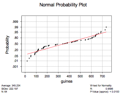
Because the data points on the normally probability plot do not adhere well to a straight line:

it suggests that the survival times are not normally distributed. We have a large sample though ( \(n=64\)). Therefore, we should be able to use the \(t\)-interval for the mean without worry. Asking Minitab to calculate the interval for us, we get:
One-Sample T: guinea
| Variable | N | Mean | StDev | SE Mean | 95.0% CI |
|---|---|---|---|---|---|
| guinea | 64 | 345.2 | 222.2 | 27.8 | (289.7, 400.7) |
That is, we can be 95% confident that the mean survival time for the population of guinea pigs is between 289.7 and 400.7 days.
Incidentally, as the following Minitab output suggests, the \(Z\)-interval for the mean is quite close to that of the \(t\)-interval for the mean:
One-Sample Z: guinea
The assumed sigma = 222.2
| Variable | N | Mean | StDev | SE Mean | 95.0% CI |
|---|---|---|---|---|---|
| guinea | 64 | 345.2 | 222.2 | 27.8 | (290.8, 399.7) |
as we would expect, because the sample is quite large.