The work on the previous page is all well and good if your probability model involves just two categories, which as we have seen, reduces to conducting a test for one proportion. What happens if our probability model involves three or more categories? It takes some theoretical work beyond the scope of this course to show it, but the chi-square statistic that we derived on the previous page can be extended to accommodate any number of k categories.
The Extension Section

Suppose an experiment can result in any of k mutually exclusive and exhaustive outcomes, say \(A_1, A_2, \dots, A_k\). If the experiment is repeated n independent times, and we let \(p_i = P(A_i)\) and \(Y_i\) = the number of times the experiment results in \(A_i, i = 1, \dots, k\), then we can summarize the number of observed outcomes and the number of expected outcomes for each of the k categories in a table as follows:
| Categories | 1 | 2 | . . . | \(k - 1\) | \(k\) |
|---|---|---|---|---|---|
| Observed | \(Y_1\) | \(Y_2\) | . . . | \(Y_{k - 1}\) | \(n - Y_1 - Y_2 - . . . - Y_{k - 1}\) |
| Expected | \(np_1\) | \(np_2\) | . . . | \(np_{k - 1}\) | \(np_k\) |
Karl Pearson showed that the chi-square statistic Q_k−1 defined as:
\[Q_{k-1}=\sum_{i=1}^{k}\frac{(Y_i - np_i)^2}{np_i} \]
follows approximately a chi-square random variable with k−1 degrees of freedom. Let's try it out on an example.
Example 16-3 Section

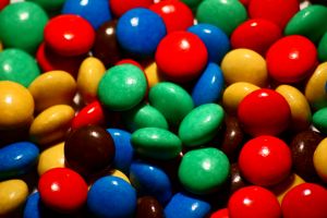
A particular brand of candy-coated chocolate comes in five different colors that we shall denote as:
- \(A_1 = \text{{brown}}\)
- \(A_2 = \text{{yellow}}\)
- \(A_3 = \text{{orange}}\)
- \(A_4 = \text{{green}}\)
- \(A_5 = \text{{coffee}}\)
Let \(p_i\) equal the probability that the color of a piece of candy selected at random belongs to \(A_i\), for \(i = 1, 2 3, 4, 5\). Test the following null and alternative hypotheses:
\(H_0 : p_{Br}=0.4,p_{Y}=0.2,p_{O}=0.2,p_{G}=0.1,p_{C}=0.1 \)
\(H_A : p_{i} \text{ not specified in null (many possible alternatives) } \)
using a random sample of n = 580 pieces of candy whose colors yielded the respective frequencies 224, 119, 130, 48, and 59. (This example comes from exercises 8.1-2 in the Hogg and Tanis (8th edition) textbook).
Answer
We can summarize the observed \((y_i)\) and expected \((np_i)\) counts in a table as follows:
| Categories | Brown | Yellow | Orange | Green | Coffee | Total |
|---|---|---|---|---|---|---|
| Observed \(y_i\) | 224 | 119 | 130 | 48 | 59 | 580 |
| Assumed \(H_0 (p_i)\) | 0.4 | 0.2 | 0.2 | 0.1 | 0.1 | 1.0 |
| Expected \(np_i\) | 232 | 116 | 116 | 58 | 58 | 580 |
where, for example, the expected number of brown candies is:
\(np_1 = 580(0.40) = 232\)
and the expected number of green candies is:
\(np_4 = 580(0.10) = 58\)
Once we have the observed and expected number of counts, the calculation of the chi-square statistic is straightforward. It is:
\(Q_4=\dfrac{(224-232)^2}{232}+d\frac{(119-116)^2}{116}+\dfrac{(130-116)^2}{116}+\dfrac{(48-58)^2}{58}+\dfrac{(59-58)^2}{58} \)
Simplifying, we get:
\(Q_4=\dfrac{64}{232}+\dfrac{9}{116}+\dfrac{196}{116}+\dfrac{100}{58}+\dfrac{1}{58}=3.784 \)
Because there are k = 5 categories, we have to compare our chi-square statistic \(Q_4\) to a chi-square distribution with k−1 = 5−1 = 4 degrees of freedom:
\(\text{Reject }H_0 \text{ if } Q_4\ge \chi_{4,0.05}^{2}=9.488\)
Because \(Q_4 = 3.784 < 9.488\), we fail to reject the null hypothesis. There is insufficient evidence at the 0.05 level to conclude that the distribution of the color of the candies differs from that specified in the null hypothesis.
By the way, this might be a good time to think about the practical meaning of the term "degrees of freedom." Recalling the example on the last page, we had two categories (male and female) and one degree of freedom. If we are sampling n = 100 people and 53 of them are female, then we absolutely must have 100−53 = 47 males. If we had instead 62 females, then we absolutely must have 100−62 = 38 males. That is, the number of females is the one number that is "free" to be any number, but once it is determined, then the number of males immediately follows. It is in this sense that we have "one degree of freedom."
With the example on this page, we have five categories of candies (brown, yellow, orange, green, coffee) and four degrees of freedom. If we are sampling n = 580 candies, and 224 are brown, 119 are yellow, 130 are orange, and 48 are green, then we absolutely must have 580−(224+119+130+48) = 59 coffee-colored candies. In this case, we have four numbers that are "free" to be any number, but once they are determined, then the number of coffee-colored candies immediately follows. It is in this sense that we have "four degrees of freedom."