Let's start our discussion of statistical power by recalling two definitions we learned when we first introduced to hypothesis testing:
- A Type I error occurs if we reject the null hypothesis \(H_0\) (in favor of the alternative hypothesis \(H_A\)) when the null hypothesis \(H_0\) is true. We denote \(\alpha=P(\text{Type I error})\).
- A Type II error occurs if we fail to reject the null hypothesis \(H_0\) when the alternative hypothesis \(H_A\) is true. We denote \(\beta=P(\text{Type II error})\).
You'll certainly need to know these two definitions inside and out, as you'll be thinking about them a lot in this lesson, and at any time in the future when you need to calculate a sample size either for yourself or for someone else.
Example 25-1 Section

The Brinell hardness scale is one of several definitions used in the field of materials science to quantify the hardness of a piece of metal. The Brinell hardness measurement of a certain type of rebar used for reinforcing concrete and masonry structures was assumed to be normally distributed with a standard deviation of 10 kilograms of force per square millimeter. Using a random sample of \(n=25\) bars, an engineer is interested in performing the following hypothesis test:
- the null hypothesis \(H_0:\mu=170\)
- against the alternative hypothesis \(H_A:\mu>170\)
If the engineer decides to reject the null hypothesis if the sample mean is 172 or greater, that is, if \(\bar{X} \ge 172 \), what is the probability that the engineer commits a Type I error?
Answer
In this case, the engineer commits a Type I error if his observed sample mean falls in the rejection region, that is, if it is 172 or greater, when the true (unknown) population mean is indeed 170. Graphically, \(\alpha\), the engineer's probability of committing a Type I error looks like this:
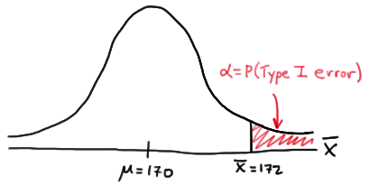
Now, we can calculate the engineer's value of \(\alpha\) by making the transformation from a normal distribution with a mean of 170 and a standard deviation of 10 to that of \(Z\), the standard normal distribution using:
\(Z= \frac{\bar{X}-\mu}{\sigma / \sqrt{n}} \)
Doing so, we get:
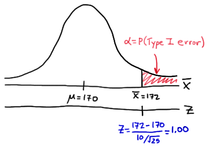
So, calculating the engineer's probability of committing a Type I error reduces to making a normal probability calculation. The probability is 0.1587 as illustrated here:
\(\alpha = P(\bar{X} \ge 172 \text { if } \mu = 170) = P(Z \ge 1.00) = 0.1587 \)
A probability of 0.1587 is a bit high. We'll learn in this lesson how the engineer could reduce his probability of committing a Type I error.
If, unknown to engineer, the true population mean were \(\mu=173\), what is the probability that the engineer commits a Type II error?
Answer
In this case, the engineer commits a Type II error if his observed sample mean does not fall in the rejection region, that is, if it is less than 172, when the true (unknown) population mean is 173. Graphically, \(\beta\), the engineer's probability of committing a Type II error looks like this:
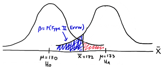
Again, we can calculate the engineer's value of \(\beta\) by making the transformation from a normal distribution with a mean of 173 and a standard deviation of 10 to that of \(Z\), the standard normal distribution. Doing so, we get:
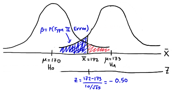
So, calculating the engineer's probability of committing a Type II error again reduces to making a normal probability calculation. The probability is 0.3085 as illustrated here:
\(\beta= P(\bar{X} < 172 \text { if } \mu = 173) = P(Z < -0.50) = 0.3085 \)
A probability of 0.3085 is a bit high. We'll learn in this lesson how the engineer could reduce his probability of committing a Type II error.
 If you think about it, considering the probability of committing a Type II error is quite similar to looking at a glass that is half empty. That is, rather than considering the probability that the engineer commits an error, perhaps we could consider the probability that the engineer makes the correct decision. Doing so, involves calculating what is called the power of the hypothesis test.
- Power of the Hypothesis Test
-
The power of a hypothesis test is the probability of making the correct decision if the alternative hypothesis is true. That is, the power of a hypothesis test is the probability of rejecting the null hypothesis \(H_0\) when the alternative hypothesis \(H_A\) is the hypothesis that is true.
Let's return to our engineer's problem to see if we can instead look at the glass as being half full!
Example 25-1 (continued) Section
If, unknown to the engineer, the true population mean were \(\mu=173\), what is the probability that the engineer makes the correct decision by rejecting the null hypothesis in favor of the alternative hypothesis?
Answer
In this case, the engineer makes the correct decision if his observed sample mean falls in the rejection region, that is, if it is greater than 172, when the true (unknown) population mean is 173. Graphically, the power of the engineer's hypothesis test looks like this:
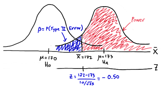
That makes the power of the engineer's hypothesis test 0.6915 as illustrated here:
\(\text{Power } = P(\bar{X} \ge 172 \text { if } \mu = 173) = P(Z \ge -0.50) = 0.6915 \)
which of course could have alternatively been calculated by simply subtracting the probability of committing a Type II error from 1, as shown here:
\(\text{Power } = 1 - \beta = 1 - 0.3085 = 0.6915 \)
At any rate, if the unknown population mean were 173, the engineer's hypothesis test would be at least a bit better than flipping a fair coin, in which he'd have but a 50% chance of choosing the correct hypothesis. In this case, he has a 69.15% chance. He could still do a bit better.
In general, for every hypothesis test that we conduct, we'll want to do the following:
-
Minimize the probability of committing a Type I error. That, is minimize \(\alpha=P(\text{Type I Error})\). Typically, a significance level of \(\alpha\le 0.10\) is desired.
-
Maximize the power (at a value of the parameter under the alternative hypothesis that is scientifically meaningful). Typically, we desire power to be 0.80 or greater. Alternatively, we could minimize \(\beta=P(\text{Type II Error})\), aiming for a type II error rate of 0.20 or less.
By the way, in the second point, what exactly does "at a value of the parameter under the alternative hypothesis that is scientifically meaningful" mean? Well, let's suppose that a medical researcher is interested in testing the null hypothesis that the mean total blood cholesterol in a population of patients is 200 mg/dl against the alternative hypothesis that the mean total blood cholesterol is greater than 200 mg/dl. Well, the alternative hypothesis contains an infinite number of possible values of the mean. Under the alternative hypothesis, the mean of the population could be, among other values, 201, 202, or 210. Suppose the medical researcher rejected the null hypothesis, because the mean was 201. Whoopdy-do...would that be a rocking conclusion? No, probably not. On the other hand, suppose the medical researcher rejected the null hypothesis, because the mean was 215. In that case, the mean is substantially different enough from the assumed mean under the null hypothesis, that we'd probably get excited about the result. In summary, in this example, we could probably all agree to consider a mean of 215 to be "scientifically meaningful," whereas we could not do the same for a mean of 201.
Now, of course, all of this talk is a bit if gibberish, because we'd never really know whether the true unknown population mean were 201 or 215, otherwise, we wouldn't have to be going through the process of conducting a hypothesis test about the mean. We can do something though. We can plan our scientific studies so that our hypothesis tests have enough power to reject the null hypothesis in favor of values of the parameter under the alternative hypothesis that are scientifically meaningful.