Before we can work on developing a hypothesis test for testing whether an empirical distribution function Fn(x) fits a hypothesized distribution function F(x) we better have a good idea of just what is an empirical distribution function Fn(x). Therefore, let's start with formally defining it.
Definition. Given an observed random sample \(X_1 , X_2 , \dots , X_n\), an empirical distribution function Fn(x) is the fraction of sample observations less than or equal to the value x. More specifically, if y1 < y2 < ... < yn are the order statistics of the observed random sample, with no two observations being equal, then the empirical distribution function is defined as:
That is, for the case in which no two observations are equal, the empirical distribution function is a "step" function that jumps 1/n in height at each observation xk. For the cases in which two (or more) observations are equal, that is, when there are nk observations at xk, the empirical distribution function is a "step" function that jumps nk/n in height at each observation xk. |
Such a formal definition is all well and good, but it would probably make even more sense if we took at a look at a simple example.
 Example
A random sample of n = 8 people yields the following (ordered) counts of the number of times they swam in the past month:
0 1 2 2 4 6 6 7
Calculate the empirical distribution function Fn(x).
As reported, the data are ordered, therefore the order statistics are y1 = 0, y2 = 1, y3 = 2, y4 = 2, y5 = 4, y6 = 6, y7 = 6, and y8 = 7. Therefore, using the definition of the empirical distribution function, we have:

and:
 and
and 
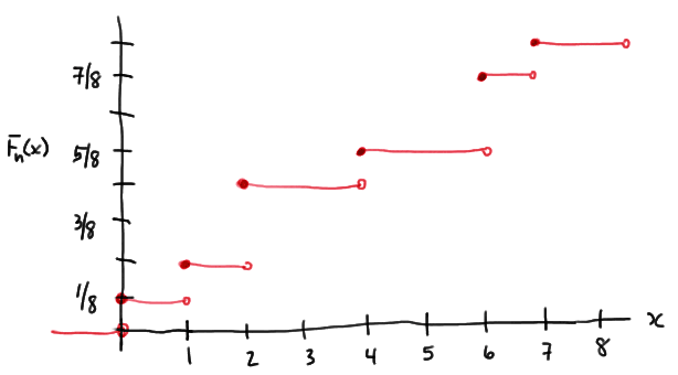
Now, noting that there are two 2s, we need to jump 2/8 at x = 2. We've already accumulated a probability of 2/8 so far. Therefore, we need to add 2/8 to it:

Then, noting that there is only one 4, we need to jump 1/8 at x = 4. That is, adding 1/8 to the 4/8 that we've already accumulated, we get:

Again, noting that there are two 6s, we need to jump 2/8 at x = 6. We've accumulated a probability of 5/8 so far. Adding 2/8 to it, we get:

And, finally:

Plotting the function, it should look something like this then:

