In one research study, 20 young pigs are assigned at random among 4 experimental groups. Each group is fed a different diet. (This design is a completely randomized design.) The data are the pigs' weights in kg after being raised on these diets for 10 months. We wish to determine if there are any differences in mean pig weights for the 4 diets.
- \(H_0: \mu_1 = \mu_2 = \mu_3 = \mu_4\)
- \(H_a:\) Not all \(\mu\) are equal
| Feed_1 | Feed_2 | Feed_3 | Feed_4 |
|---|---|---|---|
| 60.8 | 68.3 | 102.6 | 87.9 |
| 57.1 | 67.7 | 102.2 | 84.7 |
| 65.0 | 74.0 | 100.5 | 83.2 |
| 58.7 | 66.3 | 97.5 | 85.8 |
| 61.8 | 69.9 | 98.9 | 90.3 |
Contained in the Minitab file: ANOVA_ex.mpx
Note that in this file the data were entered so that each group is in its own column. In other words, the responses are in a separate column for each factor level. In later examples, you will see that Minitab will also conduct a one-way ANOVA if the responses are all in one column with the factor codes in another column.
Minitab® – One-Way ANOVA
To perform an Analysis of Variance (ANOVA) test in Minitab:
- Open the Minitab file: ANOVA_ex.mpx
- From the menu bar, select Stat > ANOVA > One-Way.
- Click the drop-down menu and select 'Responses are in a separate column for each factor level'.
- Enter the variables Feed_1, Feed_2, Feed_3, and Feed_4 to insert them into the Responses box.
- Choose the Comparisons button and check the box next to Tukey. Under Results also select Tests.
- OK and OK
The result should be the following output:
Method
| Null hypothesis | All means are equal |
|---|---|
| Alternative hypothesis | At least one mean is different |
| Significance level | \(\alpha=0.05\) |
Equal variances were assumed for the analysis
Factor Information
| Factor | Levels | Values |
|---|---|---|
| Factor | 4 | Feed_1, Feed_2, Feed_3, Feed_4 |
Analysis of Variance
| Source | DF | Adj SS | Adj MS | F-Value | P-Value |
|---|---|---|---|---|---|
| Factor | 3 | 4703.2 | 1567.73 | 206.72 | 0.000 |
| Error | 16 | 121.3 | 7.58 | ||
| Total | 19 | 4824.5 |
Model Summary
| S | R-sq | R-sq(adj) | R-sq(pred) |
|---|---|---|---|
| 2.75386 | 97.48% | 97.01% | 96.07% |
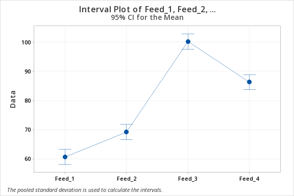
Means
| Factor | N | Mean | StDev | 95% CI |
|---|---|---|---|---|
| Feed_1 | 5 | 60.68 | 3.03 | (58.07, 63.29) |
| Feed_2 | 5 | 69.24 | 2.96 | (66.63, 71.85) |
| Feed_3 | 5 | 100.340 | 2.164 | (97.729, 102.951) |
| Feed_4 | 5 | 86.38 | 2.78 | (83.77, 88.99) |
Pooled StDev = 2.75386
Grouping Information Using the Tukey Method and 95% Confidence
| Factor | N | Mean | Grouping | |||
|---|---|---|---|---|---|---|
| Feed_3 | 5 | 100.34 | A | |||
| Feed_4 | 5 | 86.38 | B | |||
| Feed_2 | 5 | 69.24 | C | |||
| Feed_1 | 5 | 60.68 | D | |||
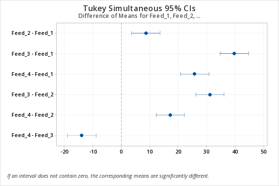
Means that do not share a letter are significantly different.
| Difference of Levels |
Difference of Means |
SE of Difference |
95% CI | T-Value | Adjusted P-Value |
|---|---|---|---|---|---|
| Feed_2 - Feed_1 | 8.56 | 1.74 | (3.57, 13.55) | 4.91 | 0.001 |
| Feed_3 - Feed_1 | 39.66 | 1.74 | (34.67, 44.65) | 22.77 | 0.000 |
| Feed_4 - Feed_1 | 25.70 | 1.74 | (20.71, 30.69) | 14.76 | 0.000 |
| Feed_3 - Feed_2 | 31.10 | 1.74 | (26.11, 36.09) | 17.86 | 0.000 |
| Feed_4 - Feed_2 | 17.14 | 1.74 | (12.15, 22.13) | 9.84 | 0.000 |
| Feed_4 - Feed_3 | -13.96 | 1.74 | (-18.95, -8.97) | -8.02 | 0.000 |
Tukey Simultaneous Tests for Differences of Means
Individual confidence level = 98.87%