Below is an example of conducting a paired means \(t\) test by hand using raw data. Next, you will learn how this can be conducted most efficiently in Minitab.
Research question: Are scores on two quizzes different?
Data were collected from 9 students and a paired means \(t\) test was performed using hand calculations:
| Student ID | Quiz 1 | Quiz 2 |
|---|---|---|
| 001 | 98 | 94 |
| 002 | 100 | 98 |
| 003 | 95 | 98 |
| 004 | 90 | 88 |
| 005 | 90 | 89 |
| 006 | 92 | 91 |
| 007 | 80 | 84 |
| 008 | 78 | 80 |
| 009 | 88 | 88 |
There are two assumptions: (1) data are paired and (2) distribution of differences is normally distribution in the population or the sample size is at least 30. The data are paired because for each student we have a quiz 1 and a quiz 2 score. We do not know if the differences are normally distributed in the population and the sample size is small, but in the video above we created a histogram of the differences and found that the sample was approximately normally distributed, so this assumption has been met and we can perform a paired means \(t\) test.
Given \(\mu_d = \mu_1 - \mu_2\), our hypotheses are:
\(H_0: \mu_d = 0\)
\(H_a: \mu_d \ne 0\)
- Test Statistic for Dependent Means
-
\(t=\frac{\bar{x}_d-\mu_0}{\frac{s_d}{\sqrt{n}}}\)
\(\overline{x}_d\) = observed sample mean difference
\(\mu_0\) = mean difference specified in the null hypothesis
\(s_d\) = standard deviation of the differences
\(n\) = sample size (i.e., number of unique individuals)
| Student ID | Quiz 1 | Quiz 2 | Difference (\(X_d\)) | \(X_d - \overline{X}_d\) | \((X_d - \overline{X}_d)^2\) |
|---|---|---|---|---|---|
| 001 | 98 | 94 | 4 | 3.889 | 15.123 |
| 002 | 100 | 98 | 2 | 1.889 | 3.568 |
| 003 | 95 | 98 | -3 | -3.111 | 9.679 |
| 004 | 90 | 88 | 2 | 1.889 | 3.568 |
| 005 | 90 | 89 | 1 | 0.889 | 0.790 |
| 006 | 92 | 91 | 1 | 0.889 | 0.790 |
| 007 | 80 | 84 | -4 | -4.111 | 16.901 |
| 008 | 78 | 80 | -2 | -2.111 | 4.457 |
| 009 | 88 | 88 | 0 | -0.111 | 0.012 |
Mean of the differences: \(\overline{X}_d=\frac{\Sigma{X}_d}{n}=\frac{1}{9}\)
For a review of computing standard deviation, see Lesson 2.
Sum of squares: \(\Sigma (X_d - \overline{X}_d)^2 = 54.889\)
Standard deviation of the differences: \(s_d=\sqrt{\frac{\sum (X_d-\overline{X}_d)^{2}}{n-1}} = \sqrt{\frac{54.889}{9-1}}=2.619\)
Test statistic: \(t=\frac{\overline{X}_d- \mu_0}{\frac{s_d}{\sqrt{n}}}=\frac{\frac{1}{9}}{\frac{2.619}{\sqrt{9}}}=0.127\)
\(df=n-1=9-1=8\)
We can construct a \(t\) distribution with 8 degrees of freedom and determine what proportion of the curve falls beyond a \(t\) score of 0.127. This is a two-tailed test, so we need to take into account both the left and right sides of the curve.
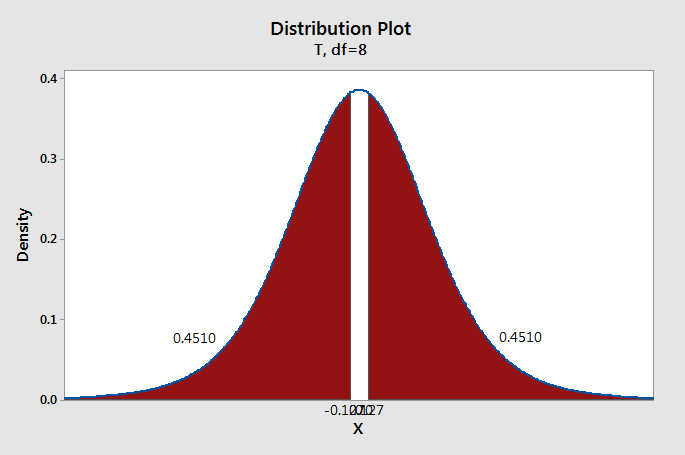
\(p=0.4510+0.4510=0.9020\)
We will compare our \(p\)-value from step 3 to a standard alpha level of 0.05.
Because \(p>\alpha\), we fail to reject the null hypothesis.
There is not sufficient evidence to state that scores on the two quizzes are different.