In a representative sample of 1168 American adults, 747 said they were not financially prepared for retirement. Let's construct a 95% confidence interval to estimate the proportion of all American adults who are not financially prepared for retirement.
First, we need to check our assumptions that both \(n\widehat p \geq 10\) and \(n(1-\widehat p) \geq 10\).
\(\widehat{p}=\frac{747}{1168}=0.640\)
\(np=1168 (0.640) = 747\) and \(n(1-p)=1168(1-0.640)=421\)
Both are greater than 10, so this assumption has been met. This means we can use the normal approximation method to construct this confidence interval.
Next, we can compute the standard error.
\(SE=\sqrt{\frac{\hat{p} (1-\hat{p})}{n}}=\sqrt{\frac{0.640 (1-0.640)}{1168}}=0.014\)
The \(z^*\) multiplier for a 95% confidence interval is 1.960
The formula for a confidence interval for a proportion is \(\widehat{p}\pm z^* (SE)\)
\(0.640\pm 1.960(0.014)=0.640\pm0.028=[0.612, \;0.668]\)
We are 95% confident that between 61.2% and 66.8% of all American adults are not financially prepared for retirement.
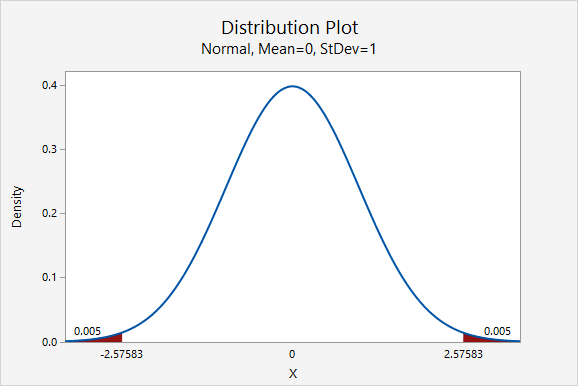
Let’s think about how our interval will change. The 99% confidence interval will be wider than the 95% confidence interval. In order to increase our level of confidence, we will need to expand the interval.
In terms of computing the 99% confidence interval, we will use the same point estimate \(\widehat{p}\) and the same standard error. Only the multiplier will change. From the plot below, we see that the \(z^*\) multiplier for a 99% confidence interval is 2.576.
\(99\%\;C.I.:\;0.640\pm 2.576 (0.014)=0.0640\pm 0.036=[0.604, \; 0.676]\)
We are 99% confidence that between 60.4% and 67.6% of all American adults are not financially prepared for retirement.