- Simple linear regression
-
A statistical method that allows us to summarize and study relationships between two continuous (quantitative) variables:
- One variable, denoted \(x\), is regarded as the predictor, explanatory, or independent variable.
- The other variable, denoted \(y\), is regarded as the response, outcome, or dependent variable.
Because the other terms are used less frequently today, we'll use the "predictor" and "response" terms to refer to the variables encountered in this course. The other terms are mentioned only to make you aware of them should you encounter them in other arenas. Simple linear regression gets its adjective "simple," because it concerns the study of only one predictor variable. In contrast, multiple linear regression, which we study later in this course, gets its adjective "multiple," because it concerns the study of two or more predictor variables.
Types of relationships Section
Before proceeding, we must clarify what types of relationships we won't study in this course, namely, deterministic (or functional) relationships. Here is an example of a deterministic relationship.
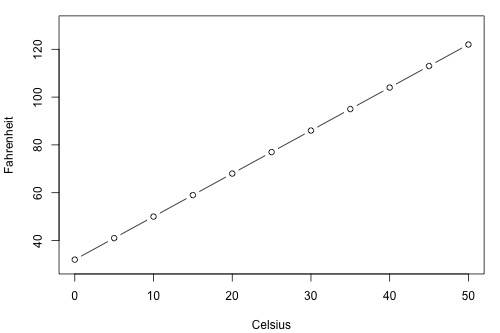
\(\text{Fahr } = \frac{9}{5}\text{Cels}+32\)
That is, if you know the temperature in degrees Celsius, you can use this equation to determine the temperature in degrees Fahrenheit exactly.
Here are some examples of other deterministic relationships that students from previous semesters have shared:
- Circumference = \(\pi\) × diameter
- Hooke's Law: \(Y = \alpha + \beta X\), where Y = amount of stretch in a spring, and X = applied weight.
- Ohm's Law: \(I = V/r\), where V = voltage applied, r = resistance, and I = current.
- Boyle's Law: For a constant temperature, \(P = \alpha/V\), where P = pressure, \(\alpha\) = constant for each gas, and V = volume of gas.
For each of these deterministic relationships, the equation exactly describes the relationship between the two variables. This course does not examine deterministic relationships. Instead, we are interested in statistical relationships, in which the relationship between the variables is not perfect.
Here is an example of a statistical relationship. The response variable y is the mortality due to skin cancer (number of deaths per 10 million people) and the predictor variable x is the latitude (degrees North) at the center of each of 48 states in the United States (U.S. Skin Cancer data) (The data were compiled in the 1950s, so Alaska and Hawaii were not yet states. And, Washington, D.C. is included in the data set even though it is not technically a state.)
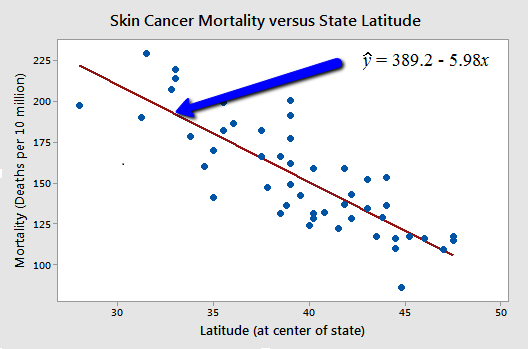
You might anticipate that if you lived in the higher latitudes of the northern U.S., the less exposed you'd be to the harmful rays of the sun, and therefore, the less risk you'd have of death due to skin cancer. The scatter plot supports such a hypothesis. There appears to be a negative linear relationship between latitude and mortality due to skin cancer, but the relationship is not perfect. Indeed, the plot exhibits some "trend," but it also exhibits some "scatter." Therefore, it is a statistical relationship, not a deterministic one.
Some other examples of statistical relationships might include:
- Height and weight — as height increases, you'd expect the weight to increase, but not perfectly.
- Alcohol consumed and blood alcohol content — as alcohol consumption increases, you'd expect one's blood alcohol content to increase, but not perfectly.
- Vital lung capacity and pack-years of smoking — as the amount of smoking increases (as quantified by the number of pack-years of smoking), you'd expect lung function (as quantified by vital lung capacity) to decrease, but not perfectly.
- Driving speed and gas mileage — as driving speed increases, you'd expect gas mileage to decrease, but not perfectly.
Okay, so let's study statistical relationships between one response variable y and one predictor variable x!