Investigating Height and GPA Data Section
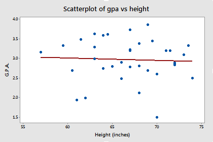
Now, let's do a similar analysis to investigate the research question, "Is there a (linear) relationship between height and grade point average?"(Height and GPA data)
Review the following scatterplot and estimated regression line. What does the plot suggest for answering the above research question? In this case, it appears as if there is almost no relationship whatsoever. The estimated slope is almost 0.
Again, we can answer the research question using the P-value of the t-test for:
- testing the null hypothesis \(H_{0} \colon \beta_{1} = 0\)
- against the alternative hypothesis \(H_{A} \colon \beta_{1} ≠ 0\).
As the Minitab output below suggests, the P-value of the t-test for "height" is 0.761. There is not enough statistical evidence to conclude that the slope is not 0. We conclude that there is no linear relationship between height and grade point average.
The Minitab output also shows the analysis of variable table for this data set. Again, the P-value associated with the analysis of variance F-test, 0.761, appears to be the same as the P-value, 0.761, for the t-test for the slope. The F-test similarly tells us that there is insufficient statistical evidence to conclude that there is a linear relationship between height and grade point average.
Analysis of Variance
| Source | DF | Adj SS | Adj MS | F-Value | P-Value |
|---|---|---|---|---|---|
| Constant | 1 | 0.0276 | 0.0276 | 0.09 | 0.761 |
| Residual Error | 33 | 9.7055 | 0.2941 | ||
| Total | 34 | 9.7331 |
Model Summary
S = 0.5423 R-Sq = 0.3% R-Sq (adj) = 0.0%
Coefficients
| Predictor | Coef | SE Coef | T-Value | P-Value |
|---|---|---|---|---|
| Constant | 3.410 | 1.435 | 2.38 | 0.023 |
| height | -0.00656 | 0.02143 | -0.31 | 0.761 |
Regression Equation
gpa = 3.14 -0.0066 height
The scatter plot of grade point average and height appear below, now adorned with the three labels:
- \(y_{i}\) denotes the observed grade point average for student i
- \(\hat{y}_i\) is the estimated regression line (solid line) and therefore denotes the estimated grade point average for the height of student i
- \(\bar{y}\) represents the "no relationship" line (dashed line) between height and grade point average. It is simply the average grade point average of the sample.
For this data set, note that the estimated regression line and the "no relationship" line are very close together. Let's see how the sums of squares summarize this point.
\(\sum_{i=1}^{n}(\hat{y}_i-\bar{y})^2 =0.0276\)
\(\sum_{i=1}^{n}(y_i-\hat{y}_i)^2 =9.7055\)
\(\sum_{i=1}^{n}(y_i-\bar{y})^2 =9.7331\)
- The "total sum of squares," which again quantifies how much the observed grade point averages vary if you don't take into account height, is \(\sum_{i=1}^{n}(y_i-\bar{y})^2 =9.7331\).
- The "regression sum of squares," which again quantifies how far the estimated regression line is from the no relationship line, is \(\sum_{i=1}^{n}(\hat{y}_i-\bar{y})^2 =0.0276\).
- The "error sum of squares," which again quantifies how much the data points vary around the estimated regression line, is \(\sum_{i=1}^{n}(y_i-\hat{y}_i)^2 =9.7055\).
In short, we have illustrated that the total variation in the observed grade point averages y (9.7331) is the sum of two parts — variation "due to" height (0.0276) and variation due to random error (9.7055). Unlike the last example, most of the variation in the observed grade point averages is just due to random error. It appears as if very little of the variation can be attributed to the predictor height.
Try It!
Sums of Squares Section
Some researchers at UCLA conducted a study on cyanotic heart disease in children. They measured the age at which the child spoke his or her first word (x, in months) and the Gesell adaptive score (y) on a sample of 21 children. Upon analyzing the resulting data, they obtained the following analysis of variance table:
Analysis of Variance
| Source | DF | Adj SS | Adj MS | F-Value | P-Value |
|---|---|---|---|---|---|
| Constant | 1 | 1604.08 | 1604.08 | 13.20 | 0.002 |
| Residual Error | 19 | 2308.59 | 121.50 | ||
| Total | 20 | 3912.67 |
Analysis of Variance
| Source | DF | Adj SS | Adj MS | F-Value | P-Value |
|---|---|---|---|---|---|
| Constant | 1 | 1604.08 | 1604.08 | 13.20 | 0.002 |
| Residual Error | 19 | 2308.59 | 121.50 | ||
| Total | 20 | 3912.67 |
Analysis of Variance
| Source | DF | Adj SS | Adj MS | F-Value | P-Value |
|---|---|---|---|---|---|
| Constant | 1 | 1604.08 | 1604.08 | 13.20 | 0.002 |
| Residual Error | 19 | 2308.59 | 121.50 | ||
| Total | 20 | 3912.67 |
Analysis of Variance
| Source | DF | Adj SS | Adj MS | F-Value | P-Value |
|---|---|---|---|---|---|
| Constant | 1 | 1604.08 | 1604.08 | 13.20 | 0.002 |
| Residual Error | 19 | 2308.59 | 121.50 | ||
| Total | 20 | 3912.67 |