Example 3-1: Hospital Infection Data Section

The hospital infection risk dataset consists of a sample of n = 58 hospitals in the east and north-central U.S. (Hospital Infection Data Region 1 and 2 data). The response variable is y = infection risk (percent of patients who get an infection) and the predictor variable is x = average length of stay (in days). Minitab output for a simple linear regression model fit to these data follows:
Regression Analysis: InfctRsk versus Stay
Analysis of Variance
| Source | DF | Adj SS | Adj Ms | F-Value | P-Value |
|---|---|---|---|---|---|
| Regression | 1 | 38.3059 | 38.3059 | 36.50 | 0.000 |
| Stay | 1 | 38.3059 | 38.3059 | 36.50 | 0.000 |
| Error | 56 | 58.7763 | 1.0496 | ||
| Lack-of-Fit | 54 | 58.5513 | 1.0843 | 9.64 | 0.098 |
| Pure error | 2 | 0.2250 | 0.1125 | ||
| Total | 57 | 97.0822 |
Model Summary
| S | R-Sq | R-Sq (adj) | R-Sq (pred) |
|---|---|---|---|
| 1.02449 | 39.46% | 38.38% | 35.07% |
Coefficients
| Term | Coef | SE Coef | T-Value | P-Value | VIF |
|---|---|---|---|---|---|
| Constant | -1.160 | 0.956 | -1.21 | 0.230 | |
| Stay | 0.5689 | 0.0942 | 6.04 | 0.000 | 1.00 |
Regression Equation
InfctRsk = -1.160 + 0.5689 Stay
Minitab output with information for x = 10.
Prediction for InfctRsk
Regression Equation
InfctRsk = -1.160 + 0.5689 Stay
| Variable | Setting |
|---|---|
| Stay | 10 |
| Fit | SE Fit | 95% CI | 95% PI |
|---|---|---|---|
| 4.52885 | 0.134602 | (4.25921, 4.79849) | (2.45891, 6.59878) |
We can make the following observations:
- For the interval given under 95% CI, we say with 95% confidence we can estimate that in hospitals in which the average length of stay is 10 days, the mean infection risk is between 4.25921 and 4.79849.
- For the interval given under 95% PI, we say with 95% confidence that for any future hospital where the average length of stay is 10 days, the infection risk is between 2.45891 and 6.59878.
- The value under Fit is calculated as \(\hat{y} = −1.160 + 0.5689(10) = 4.529\).
- The value under SE Fit is the standard error of \(\hat{y}\) and it measures the accuracy of \(\hat{y}\) as an estimate of E(Y ).
- Since df = n − 2 = 58 − 2 = 56, the multiplier for 95% confidence is 2.00324. The 95% CI for E(Y) is calculated as \begin{align} &=4.52885 \pm (2.00324 × 0.134602)\\ &= 4.52885 \pm 0.26964\\ &= (4.259, 4.798)\end{align}
- Since S = \(\sqrt{MSE}\) = 1.02449, the 95% PI is calculated as \begin{align} &=4.52885 \pm (2.00324 × \sqrt{1.02449^2 + 0.134602^2})\\ &= 4.52885 \pm 2.0699 = (2.459, 6.599)\end{align}
The following figure provides plots showing the difference between the confidence intervals (CI) and prediction intervals (PI) we have been considering.
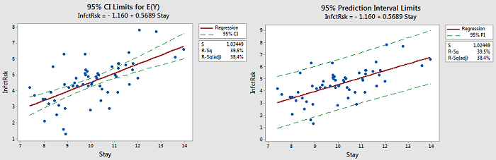
There are also some things to note:
- Notice that the limits for E(Y) are close to the line. The purpose of those limits is to estimate the "true" location of the line.
- Notice that the prediction limits (on the right) bracket most of the data. Those limits describe the location of individual y-values.
- Notice that the prediction intervals are wider than the confidence intervals. This is something that can be noted by the formulas.