In this section, we learn how to use residuals versus fits (or predictor) plots to detect problems with our formulated regression model. Specifically, we investigate:
- how a non-linear regression function shows up on a residuals vs. fits plot
- how unequal error variances show up on a residuals vs. fits plot
- how an outlier shows up on a residuals vs. fits plot.
Example Is tire tread wear linearly related to mileage? A laboratory (Smith Scientific Services, Akron, OH) conducted an experiment in order to answer this research question. As a result of the experiment, the researchers obtained a data set (Treadwear data) containing the mileage (x, in 1000 miles) driven and the depth of the remaining groove (y, in mils). The fitted line plot of the resulting data:
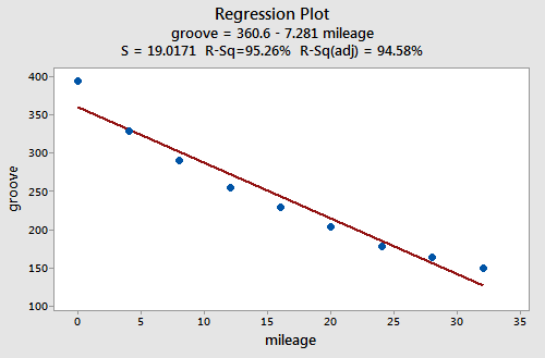
suggests that there is a relationship between groove depth and mileage. The relationship is just not linear. As is generally the case, the corresponding residuals vs. fits plot accentuates this claim:
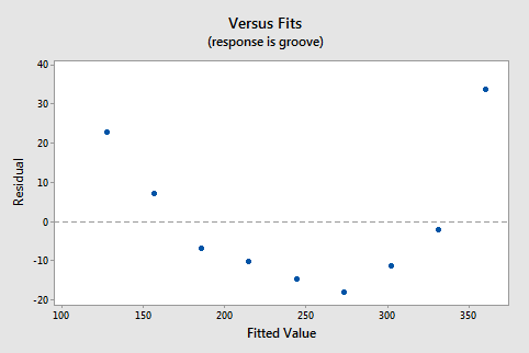
Incidentally, did you notice that the \(r^2\) value is very high (95.26%)? This is an excellent example of the caution that "a large \(r^2\) value should not be interpreted as meaning that the estimated regression line fits the data well." The large \(r^2\) value tells you that if you wanted to predict groove depth, you'd be better off taking into account mileage than not. The residuals vs. fits plot tells you, though, that your prediction would be better if you formulated a non-linear model rather than a linear one.
Answer:
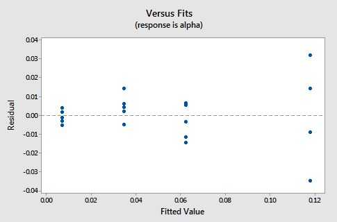
Non-constant error variance shows up on a residuals vs. fits (or predictor) plot in any of the following ways:
- The plot has a "fanning" effect. That is, the residuals are close to 0 for small x values and are more spread out for large x values.
- The plot has a "funneling" effect. That is, the residuals are spread out for small x values and close to 0 for large x values.
- Or, the spread of the residuals in the residuals vs. fits plot varies in some complex fashion.
An Example: How is plutonium activity related to alpha particle counts? Plutonium emits subatomic particles — called alpha particles. Devices used to detect plutonium record the intensity of alpha particle strikes in counts per second. To investigate the relationship between plutonium activity (x, in pCi/g) and alpha count rate (y, in number per second), a study was conducted on 23 samples of plutonium. The following fitted line plot was obtained on the resulting data (Alpha Pluto dataset):
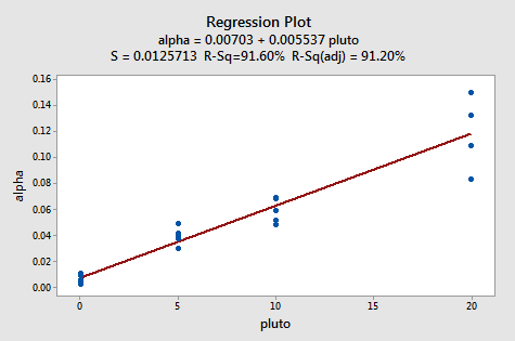
The plot suggests that there is a linear relationship between alpha count rate and plutonium activity. It also suggests that the error terms vary around the regression line in a non-constant manner — as the plutonium level increases, not only does the mean alpha count rate increase, but also the variance increases. That is, the fitted line plot suggests that the assumption of equal variances is violated. As is generally the case, the corresponding residuals vs. fits plot accentuates this claim:
Answer:
The observation's residual stands apart from the basic random pattern of the rest of the residuals. The random pattern of the residual plot can even disappear if one outlier really deviates from the pattern of the rest of the data.
An Example: Is there a relationship between tobacco use and alcohol use? The British government regularly conducts surveys on household spending. One such survey (Family Expenditure Survey, Department of Employment, 1981) determined the average weekly expenditure on tobacco (x, in British pounds) and the average weekly expenditure on alcohol (y, in British pounds) for households in n = 11 different regions in the United Kingdom. The fitted line plot of the resulting data (Alcohol Tobacco dataset):
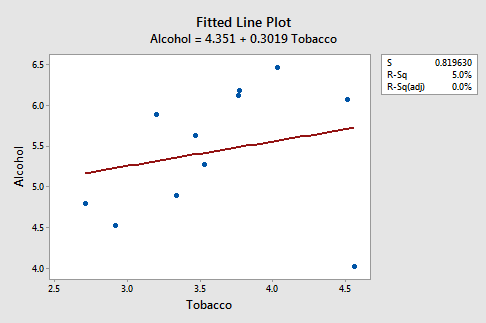
suggests that there is an outlier — in the lower right corner of the plot — which corresponds to the Northern Ireland region. In fact, the outlier is so far removed from the pattern of the rest of the data that it appears to be "pulling the line" in its direction. As is generally the case, the corresponding residuals vs. fits plot accentuates this claim:
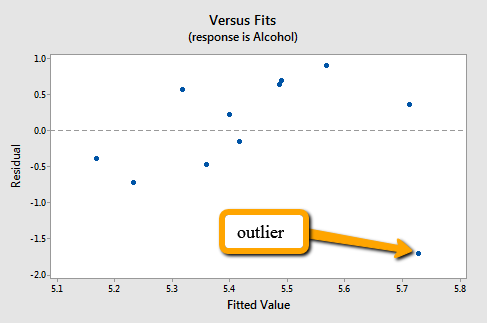
Note that Northern Ireland's residual stands apart from the basic random pattern of the rest of the residuals. That is, the residual vs. fits plot suggests that an outlier exists.
Incidentally, this is an excellent example of the caution that the "coefficient of determination \(r^2\) can be greatly affected by just one data point." Note above that the \(r^2\) value on the data set with all n = 11 regions included is 5%. Removing Northern Ireland's data point from the data set, and refitting the regression line, we obtain:
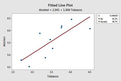
The \(r^2\) value has jumped from 5% ("no-relationship") to 61.5% (" moderate relationship")! Can one data point greatly affect the value of \(r^2\)? Clearly, it can!
Now, you might be wondering how large a residual has to be before a data point should be flagged as being an outlier. The answer is not straightforward, since the magnitude of the residuals depends on the units of the response variable. That is, if your measurements are made in pounds, then the units of the residuals are in pounds. And, if your measurements are made in inches, then the units of the residuals are in inches. Therefore, there is no one "rule of thumb" that we can define to flag a residual as being exceptionally unusual.
There's a solution to this problem. We can make the residuals "unitless" by dividing them by their standard deviation. In this way, we create what is called "standardized residuals." They tell us how many standard deviations above — if positive — or below — if negative — a data point is from the estimated regression line.
The corresponding standardized residuals vs. fits plot for our expenditure survey example looks like this:
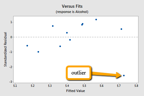
The standardized residual of the suspicious data point is smaller than -2. That is, the data point lies more than 2 standard deviations below its mean. Since this is such a small dataset the data point should be flagged for further investigation!
Incidentally, Minitab (and most other statistical software) identifies observations with large standardized residuals. Here is what a portion of Minitab's output for our expenditure survey example looks like:
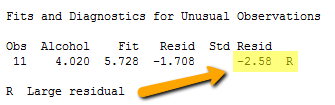
Minitab labels observations with large standardized residuals with an "R." For our example, Minitab reports that observation #11 — for which tobacco = 4.56 and alcohol = 4.02 — has a large standardized residual (-2.58). The data point has been flagged for further investigation.
Note! that I have intentionally used the phrase "flagged for futher investigation." I have not said that the data point should be "removed." Here's my recommended strategy, once you've identified a data point as being unusual:
- Determine whether a simple and therefore correctable, mistake was made in recording or entering the data point. Examples include transcription errors (recording 62.1 instead of 26.1) or data entry errors (entering 99.1 instead of 9.1). Correct the mistakes you found.
- Determine if the measurement was made in such a way that keeping the experimental unit in the study can no longer be justified. Was some procedure not conducted according to study guidelines? For example, was a person's blood pressure measured standing up rather than sitting down? Was the measurement made on someone not in the population of interest? For example, was the survey completed by a man instead of a woman? If it is convincingly justifiable, remove the data point from the data set.
- If the first two steps don't resolve the problem, consider analyzing the data twice — once with the data point included and once with the data point excluded. Report the results of both analyses.