Example 6-4: Peruvian Blood Pressure Data Section

This dataset consists of variables possibly relating to blood pressures of n = 39 Peruvians who have moved from rural high-altitude areas to urban lower-altitude areas (Peru data). The variables in this dataset are:
\(Y\) = systolic blood pressure
\(X_{1}\) = age
\(X_{2}\) = years in urban area
\(X_{3}\) = \(X_{2}\) /\(X_{1}\) = fraction of life in urban area
\(X_{4}\) = weight (kg)
\(X_{5}\) = height (mm)
\(X_{6}\) = chin skinfold
\(X_{7}\) = forearm skinfold
\(X_{8}\) = calf skinfold
\(X_{9}\) = resting pulse rate
First, we run a multiple regression using all nine x-variables as predictors. The results are given below.
Analysis of Variance
| Source | DF | Adj SS | Adj MS | F- Value | P-Value |
|---|---|---|---|---|---|
| Regression | 9 | 4358.85 | 484.32 | 6.46 | 0.000 |
| Error | 29 | 2172.58 | 74.92 | ||
| Total | 38 | 6531.44 |
Model Summary
| S | R-sq | R-sq(adj) | R-sq(pred) |
|---|---|---|---|
| 8.65544 | 66.74% | 56.41% | 34.45% |
Coefficients
| Term | Coef | SE Coef | T-Value | P-Value | VIF |
|---|---|---|---|---|---|
| Constant | 146.8 | 49.0 | 3.00 | 0.006 | |
| Age | -1.121 | 0.327 | -.343 | 0.002 | 3.21 |
| Years | 2.455 | 0.815 | 3.01 | 0.005 | 34.29 |
| FracLife | -115.3 | 30.2 | -3.82 | 0.001 | 24.39 |
| Weight | 1.414 | 0.431 | 3.28 | 0.003 | 4.75 |
| Height | -0.0346 | 0.0369 | -0.94 | 0.355 | 1.91 |
| Chin | -0.944 | 0.741 | -1.27 | 0.213 | 2.06 |
| Forearm | -1.17 | 1.19 | -0.98 | 0.335 | 3.80 |
| Calf | -0.159 | 0.537 | -0.30 | 0.770 | 2.41 |
| Pulse | 0.115 | 0.170 | 0.67 | 0.507 | 1.33 |
When looking at tests for individual variables, we see that p-values for the variables Height, Chin, Forearm, Calf, and Pulse are not at a statistically significant level. These individual tests are affected by correlations amongst the x-variables, so we will use the General Linear F procedure to see whether it is reasonable to declare that all five non-significant variables can be dropped from the model.
Next, consider testing:
\(H_{0} \colon \beta_5 = \beta_6 = \beta_7 = \beta_8 = \beta_9 = 0\)
\(H_{A} \colon\)at least one of \(\beta_5 , \beta_6 , \beta_7, \beta_8 , \beta_9 \ne 0\)
within the nine-variable model given above. If this null is not rejected, it is reasonable to say that none of the five variables Height, Chin, Forearm, Calf, and Pulse contribute to the prediction/explanation of systolic blood pressure.
The full model includes all nine variables; SSE(full) = 2172.58, the full error df = 29, and MSE(full) = 74.92 (we get these from the Minitab results above). The reduced model includes only the variables Age, Years, fraclife, and Weight (which are the remaining variables if the five possibly non-significant variables are dropped). Regression results for the reduced model are given below.
Analysis of Variance
| Source | DF | Adj SS | Adj MS | F- Value | P-Value |
|---|---|---|---|---|---|
| Regression | 4 | 3901.7 | 975.43 | 12.61 | 0.000 |
| Error | 34 | 2629.7 | 77.34 | ||
| Total | 38 | 6531.4 |
Model Summary
| S | R-sq | R-sq(adj) | R-sq(pred) |
|---|---|---|---|
| 8.79456 | 59.74% | 55.00% | 44.84% |
Coefficients
| Term | Coef | SE Coef | T-Value | P-Value | VIF |
|---|---|---|---|---|---|
| Constant | 116.8 | 22.0 | 5.32 | 0.000 | |
| Age | -0.951 | 0.316 | -3.00 | 0.005 | 2.91 |
| Years | 2.339 | 0.771 | 3.03 | 0.005 | 29.79 |
| FracLife | -108.1 | 28.3 | -3.81 | 0.001 | 20.83 |
| Weight | 0.832 | 0.275 | 3.02 | 0.005 | 1.88 |
We see that SSE(reduced) = 2629.7, and the reduced error df = 34. We also see that all four individual x-variables are statistically significant.
The calculation for the general linear F-test statistic is:
\(F=\dfrac{\frac{\text{SSE(reduced) - SSE(full)}}{\text{error df for reduced - error df for full}}}{\text{MSE(full)}}=\dfrac{\frac{2629.7-2172.58}{34-29}}{74.92}=1.220\)
Thus, this test statistic comes from an \(F_{5,29}\) distribution, of which the associated p-value is 0.325 (this can be done by using Calc >> Probability Distribution >> F in Minitab). This is not at a statistically significant level, so we do not reject the null hypothesis. Thus it is feasible to drop the variables \(X_{5}\), \(X_{6}\), \(X_{7}\), \(X_{8}\), and \(X_{9 }\) from the model.
Video: Testing a Subset of Predictors in a Multiple Linear Regression Model
Example 6-5: Measurements of College Students Section
For n = 55 college students, we have measurements (Physical dataset) for the following five variables:
\(Y\) = height (in)
\(X_{1 }\)= left forearm length (cm)
\(X_{2 }\)= left foot length (cm)
\(X_{3 }\)= head circumference (cm)
\(X_{4 }\)= nose length (cm)
The Minitab output for the full model is given below.
Coefficients
| Term | Coef | SE Coef | 95% CI | T-Value | P-Value | VIF |
|---|---|---|---|---|---|---|
| Constant | 18.50 | 7.83 | ( 2.78, 34.23) | 2.36 | 0.022 | |
| LeftArm | 0.802 | 0.171 | ( 0.459, 1.145) | 4.70 | 0.000 | 1.63 |
| LeftFoot | 0.997 | 0.162 | ( 0.671, 1.323) | 6.14 | 0.000 | 1.28 |
| HeadCirc | 0.081 | 0.150 | (-0.220, 0.381) | 0.54 | 0.593 | 1.28 |
| nose | -0.147 | 0.492 | (-1.136, 0.841) | -0.30 | 0.766 | 1.14 |
Regression Equation
Height = 18.50 + 0.802 LeftArm + 0.997 LeftFoot + 0.081 HeadCirc - 0.147 nose
Notice in the output that there are also t-test results provided. The interpretations of these t-tests are as follows:
- The sample coefficients for LeftArm and LeftFoot achieve statistical significance. This indicates that they are useful as predictors of Height.
- The sample coefficients for HeadCirc and nose are not significant. Each t-test considers the question of whether the variable is needed, given that all other variables will remain in the model.
Below is a plot of residuals versus the fitted values and it seems suitable.
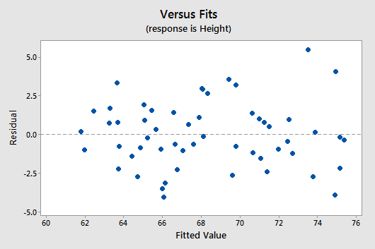
There is no obvious curvature and the variance is reasonably constant. One may note two possible outliers, but nothing serious.
The first calculation we will perform is for the general linear F-test. The results above might lead us to test
\(H_{0} \colon \beta_3 = \beta_4 = 0\)
\(H_{A} \colon\) at least one of \(\left( \beta_3 , \beta_4 \right) \ne 0\)
in the full model. If we fail to reject the null hypothesis, we could then remove both of HeadCirc and nose as predictors.
Below is the ANOVA table for the full model.
Analysis of Variance
| Source | DF | Seq SS | Seq MS | F- Value | P-Value |
|---|---|---|---|---|---|
| Regression | 4 | 816.39 | 204.098 | 42.81 | 0.000 |
| LeftArm | 1 | 590.21 | 590.214 | 123.81 | 0.000 |
| LeftFoot | 1 | 224.35 | 224.349 | 47.06 | 0.000 |
| headCirc | 1 | 1.40 | 1.402 | 0.29 | 0.590 |
| nose | 1 | 0.43 | 0.427 | 0.09 | 0.766 |
| Error | 50 | 238.35 | 4.767 | ||
| Total | 54 | 1054.75 |
From this output, we see that SSE(full) = 238.35, with df = 50, and MSE(full) = 4.77. The reduced model includes only the two variables LeftArm and LeftFoot as predictors. The ANOVA results for the reduced model are found below.
Analysis of Variance
| Source | DF | Seq SS | Seq MS | F- Value | P-Value |
|---|---|---|---|---|---|
| Regression | 2 | 814.56 | 407.281 | 88.18 | 0.000 |
| LeftArm | 1 | 590.21 | 590214 | 127.78 | 0.000 |
| LeftFoot | 1 | 224.35 | 224.349 | 48.57 | 0.000 |
| Error | 52 | 240.18 | 4.619 | ||
| Lack-of-Fit | 44 | 175.14 | 3.980 | 0.49 | 0.937 |
| Pure Error | 8 | 65.04 | 8.130 | ||
| Total | 54 | 1054.75 |
From this output, we see that SSE(reduced) = SSE\(\left( X_{1} , X_{2}\right)\) = 240.18, with df = 52, and MSE(reduced) = MSE\(\left(X_{1}, X_{2}\right) = 4.62\).
With these values obtained, we can now obtain the test statistic for testing \(H_{0} \colon \beta_3 = \beta_4 = 0\):
\(F=\dfrac{\frac{\text{SSE}(X_1, X_2) - \text{SSE(full)}}{\text{error df for reduced - error df for full}}}{\text{MSE(full)}}=\dfrac{\frac{240.18-238.35}{52-50}}{4.77}=0.192\)
This value comes from an \(F_{2,50}\) distribution. By using Calc >> Probability Distribution >> F in Minitab, we learn that the area to the left of F = 0.192 (with df of 2 and 50) is 0.174. The p-value is the area to the right of F, so p = 1 − 0.174 = 0.826. Thus, we do not reject the null hypothesis and it is reasonable to remove HeadCirc and nose from the model.
Next we consider what fraction of variation in Y = Height cannot be explained by \(X_{2}\) = LeftFoot, but can be explained by \(X_{1}\) = LeftArm? To answer this question, we calculate the partial \(R^{2}\). The formula is:
\(R_{Y, 1|2}^{2}=\dfrac{SSR(X_1|X_2)}{SSE(X_2)}=\dfrac{SSE(X_2)-SSE(X_1,X_2)}{SSE(X_2)}\)
The denominator, SSE\(\left(X_{2}\right)\), measures the unexplained variation in Y when \(X_{2 }\)is the predictor. The ANOVA table for this regression is found below.
Analysis of Variance
| Source | DF | Seq SS | Seq MS | F- Value | P-Value |
|---|---|---|---|---|---|
| Regression | 1 | 707.4 | 707.420 | 107.95 | 0.000 |
| LeftFoot | 1 | 707.4 | 707.420 | 107.95 | 0.000 |
| Error | 53 | 347.3 | 6.553 | ||
| Lack-of-Fit | 19 | 113.0 | 5.948 | 0.86 | 0.625 |
| Pure Error | 34 | 234.3 | 6.892 | ||
| Total | 54 | 1054.7 |
These results give us SSE\(\left(X_{2}\right)\) = 347.3.
The numerator, SSE\(\left(X_{2}\right)\)–SSE\(\left(X_{1}, X_{2}\right)\), measures the further reduction in the SSE when \(X_{1}\) is added to the model. Results from the earlier Minitab output give us SSE\(\left(X_{1} , X_{2}\right)\) = 240.18 and now we can calculate:
\begin{align}R_{Y, 1|2}^{2}&=\dfrac{SSR(X_1|X_2)}{SSE(X_2)}=\dfrac{SSE(X_2)-SSE(X_1,X_2)}{SSE(X_2)}\\&=\dfrac{347.3-240.18}{347.3}=0.308\end{align}
Thus \(X_{1}\)= LeftArm explains 30.8% of the variation in Y = Height that could not be explained by \(X_{2}\) = LeftFoot.