In this section, we focus on issues concerning the coding of qualitative variables. In particular, we:
- learn a general rule for the number of indicator variables that are necessary for coding a qualitative variable
- investigate the impact of using a different coding scheme, such as (1, -1) coding, on the interpretation of the regression coefficients
A general rule for coding a qualitative variable
In the birth weight example, we coded the qualitative variable Smoking by creating a (0, 1) indicator variable that took on the value 1 for smoking mothers and 0 for non-smoking mothers. What if we had instead tried to use two indicator variables? That is, what if we created one (0, 1) indicator variable, \(x_{i2}\) say, for smoking mothers defined as:
- \(x_{i2} = 1\), if mother smokes
- \(x_{i2} = 0\), if mother does not smoke
and one (0, 1) indicator variable, \(x_{i3}\) say, for non-smoking mothers defined as:
- \(x_{i3} = 1\), if mother does not smoke
- \(x_{i3} = 0\), if mother smokes
In this case, our modified regression function with two binary predictors and one quantitative predictor would be:
\(\mu_Y=\beta_0+\beta_1x_{i1}+\beta_2x_{i2}+\beta_3x_{i3}\)
where:
- \(\mu_{Y}\) is the mean birth weight for given predictors
- \(x_{i1}\) is the length of gestation of baby i
- \(x_{i2} = 1\), if mother smokes and \(x_{i2} = 0\), if mother does not
- \(x_{i3} = 1\), if mother does not smoke and \(x_{i3} = 0\), if mother smokes
Do you see where this is going? Let's see what the implication of such a coding scheme is on the data analysis:
Regression Analysis: Weight versus gest, x2*, x3*
* x3* is highly correlated with other X variables
* x3* has been removed from the equation
The regression equation is
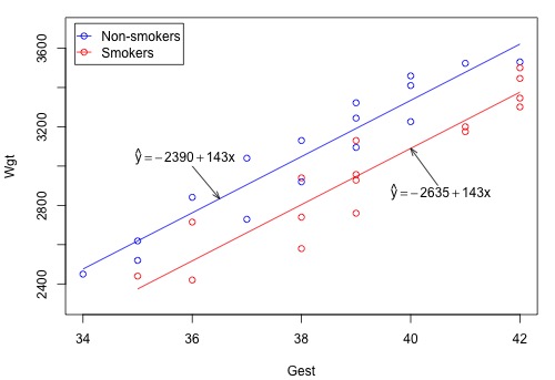
Weight = -2390 + 143 Gest - 245 x2*
| Predictor | Coef | SE Coef | T | P |
|---|---|---|---|---|
| Constant | -2389.6 | 349.2 | -6.84 | 0.000 |
| Gest | -143.100 | 9.128 | 15.68 | 0.000 |
| x2* | -244.54 | 41.98 | -5.83 | 0.000 |
| Modal Summary | ||
|---|---|---|
| S = 115.5 | R-Sq = 89.6% | R-Sq(adj) = 88.9% |
As you can see in blue, Minitab has problems with fitting the model. This is not a problem unique to Minitab — any statistical software would have problems. At issue is that the indicator variable \(x_{3}\) is "highly correlated" with the indicator variable \(x_{2}\) . In fact, \(x_{2}\) and \(x_{3}\) are perfectly correlated with one another — when \(x_{2}\) is 1, \(x_{3}\) is always 0 and when \(x_{2}\) is 0, \(x_{3}\) is always 1. (Described more technically, the columns of the X matrix are linearly dependent — if you add the \(x_{2}\) and \(x_{3}\) columns you get the column of 1's for the intercept term.) As you can see ("x3 has been removed from the equation"), Minitab attempts to fix the problem for us by dropping from the model the last predictor variable listed.
How do we prevent such problems from occurring when coding a qualitative variable? The short answer is to always create one fewer indicator variable than the number of groups defined by the qualitative variable. That is, in general, a qualitative variable defining c groups should be represented by c - 1 indicator variables, each taking on values 0 and 1. For example:
- If your qualitative variable defines 2 groups, then you need 1 indicator variable.
- If your qualitative variable defines 3 groups, then you need 2 indicator variables.
- If your qualitative variable defines 4 groups, then you need 3 indicator variables.
And, so on.
Then, choose one group or category to be the "reference" group (often it will be clear from the application which group should be the reference group, such as a control group in a medical experiment, but, if not, then the group with the most observations is often a good choice; if all groups are the same size and there is no obvious reference group then simply select the most convenient group). Observations in this group will have the value zero for all the indicator variables used to code this qualitative variable. Each of the remaining c – 1 groups will be represented by one and only one of the c – 1 indicator variables. For examples of how this works in practice, see the three-group examples in Section 6.1, where "no cooling" is the reference group, and Section 8.6, where treatment C is the reference group.
The impact of using a different coding scheme
In the birth weight example, we coded the qualitative variable Smoking by creating a (0, 1) indicator variable that took on the value 1 for smoking mothers and 0 for non-smoking mothers. What if we had instead used (1, -1) coding? That is, what if we created a (1, -1) indicator variable, \(x_{i2}\) say, defined as:
- \(x_{i2} = 1\), if the mother smokes
- \(x_{i2} = -1\), if mother does not smoke
In this case, our modified regression function using a (1, -1) coding scheme would be:
\(y_i=(\beta_0+\beta_1x_{i1}+\beta_2x_{i2})+\epsilon_i\)
where:
- \(y_{i}\) is the birth weight of baby i
- \(x_{i1}\) is the length of gestation of baby i
- \(x_{i2} = 1\), if the mother smokes and \(x_{i2} = -1\), if the mother does not smoke
The mean response function:
\(\mu_Y=\beta_0+\beta_1x_{i1}+\beta_2x_{i2}\)
yields two different response functions. If the mother is a non-smoker, then \(x_{i2} = -1\) and the mean response function looks like:
\(\mu_Y=(\beta_0-\beta_2)+\beta_1x_{i1}\)
while if the mother is a smoker, then \(x_{i2} = 1\) and the mean response function looks like this:
\(\mu_Y=(\beta_0+\beta_2)+\beta_1x_{i1}\)
Recall that the fundamental principle is that you can determine the meaning of any regression coefficient by seeing what effect changing the value of the predictor has on the mean response \(\mu_{Y}\). Here's the interpretation of the regression coefficients in a regression model with one (1, -1) binary indicator variable and one quantitative predictor, as well as an illustration of how the meaning was determined:
- \(\beta_{1}\) represents the change in the mean response \(\mu_{Y}\) for each additional unit increase in the quantitative predictor \(x_{1}\) for both groups. Note that the interpretation of this slope parameter is no different than the interpretation when using (0, 1) coding.
- \(\beta_{0}\) represents the overall "average" intercept ignoring group.
- \(\beta_{2}\) represents how far each group is "offset" from the overall "average"
Using the (1, -1) coding scheme, Minitab tells us:
Regression equation
Weight = -2512 + 143 Gest - 122 Smoking2The estimate of the smoking parameter, -122, tells us that each group is "offset" from the overall "average" by 122 grams. And, if each group is offset from the overall average by 122 grams, then the estimate of the difference in the mean weights of the two groups must be 122+122 or 244 grams. Recall that the estimated smoking coefficient obtained when using the (0, 1) coding scheme was -245:
Regression equation
Weight = - 2390 + 143 Gest - 245 Smokingtelling us that the difference in the mean weights of the two groups is 245 grams. Makes sense? (The fact that the estimated coefficient is -245 rather than -244 is just due to the rounding that Minitab uses when reporting the equations.)
If we set Smoking2 once equal to -1 and once equal to 1, we obtain the same two distinct estimated lines:
In short, regardless of the coding scheme used, we obtain the same two estimated functions and draw the same scientific conclusions. It's just how we arrive at those conclusions that differ. The meanings of the regression coefficients differ. That's why it is fundamentally critical that you not only keep track of how you code your qualitative variables but also can figure out how your coding scheme impacts the interpretation of the regression coefficients. Furthermore, when reporting your results, you should make sure you explain the coding scheme you used. And, when interpreting others' results, you should make sure you know what coding scheme they used!