In our earlier discussions on multiple linear regression, we have outlined ways to check assumptions of linearity by looking for curvature in various plots.
- For instance, we look at the scatterplot of the residuals versus the fitted values.
- We also look at a scatterplot of the residuals versus each predictor.
Sometimes, a plot of the residuals versus a predictor may suggest there is a nonlinear relationship. One way to try to account for such a relationship is through a polynomial regression model. Such a model for a single predictor, X, is:
\(\begin{equation}\label{poly} Y=\beta _{0}+\beta _{1}X +\beta_{2}X^{2}+\ldots+\beta_{h}X^{h}+\epsilon, \end{equation}\)
where h is called the degree of the polynomial. For lower degrees, the relationship has a specific name (i.e., h = 2 is called quadratic, h = 3 is called cubic, h = 4 is called quartic, and so on). Although this model allows for a nonlinear relationship between Y and X, polynomial regression is still considered linear regression since it is linear in the regression coefficients, \(\beta_1, \beta_2, ..., \beta_h\)!
In order to estimate the equation above, we would only need the response variable (Y) and the predictor variable (X). However, polynomial regression models may have other predictor variables in them as well, which could lead to interaction terms. So as you can see, the basic equation for a polynomial regression model above is a relatively simple model, but you can imagine how the model can grow depending on your situation!
For the most part, we implement the same analysis procedures as done in multiple linear regression. To see how this fits into the multiple linear regression framework, let us consider a very simple data set of size n = 50 that was simulated:
| i | \(x_i\) | \(y_i\) | i | \(x_i\) | \(y_i\) | i | \(x_i\) | \(y_i\) |
|---|---|---|---|---|---|---|---|---|
| 1 | 6.6 | -45.4 | 21 | 8.4 | -106.5 | 41 | 8 | -95.8 |
| 2 | 10.1 | -176.6 | 22 | 7.2 | -63 | 42 | 8.9 | -126.2 |
| 3 | 8.9 | -127.1 | 23 | 13.2 | -362.2 | 43 | 10.1 | -179.5 |
| 4 | 6 | -31.1 | 24 | 7.1 | -61 | 44 | 11.5 | -252.6 |
| 5 | 13.3 | -366.6 | 25 | 10.4 | -194 | 45 | 12.9 | -338.5 |
| 6 | 6.9 | -53.3 | 26 | 10.8 | -216.4 | 4 | 8.1 | -97.3 |
| 7 | 9 | -131.1 | 27 | 11.9 | -278.1 | 47 | 14.9 | -480.5 |
| 8 | 12.6 | -320.9 | 28 | 9.7 | -162.7 | 48 | 13.7 | -393.6 |
| 9 | 10.6 | -204.8 | 29 | 5.4 | -21.3 | 49 | 7.8 | -87.6 |
| 10 | 10.3 | -189.2 | 30 | 12.1 | -284.8 | 50 | 8.5 | -105.4 |
| 11 | 14.1 | -421.2 | 31 | 12.1 | -287.5 | |||
| 12 | 8.6 | -113.1 | 32 | 12.1 | -290.8 | |||
| 13 | 14.9 | -482.3 | 33 | 9.2 | -137.4 | |||
| 14 | 6.5 | -42.9 | 34 | 6.7 | -47.7 | |||
| 15 | 9.3 | -144.8 | 35 | 12.1 | -292.3 | |||
| 16 | 5.2 | -14.2 | 36 | 13.2 | -356.4 | |||
| 17 | 10.7 | -211.3 | 37 | 11 | -228.5 | |||
| 18 | 7.5 | -75.4 | 38 | 13.1 | -354.4 | |||
| 19 | 14.9 | -482.7 | 39 | 9.2 | -137.2 | |||
| 20 | 12.2 | -295.6 | 40 | 13.2 | -361.6 |
The data was generated from the quadratic model
\(\begin{equation} y_{i}=5+12x_{i}-3x_{i}^{2}+\epsilon_{i}, \end{equation}\)
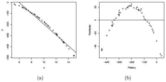
where the \(\epsilon_{i}s\) are assumed to be normally distributed with mean 0 and variance 2. A scatterplot of the data along with the fitted simple linear regression line is given below. As you can see, a linear regression line is not a reasonable fit to the data.


(a) Scatterplot of the quadratic data with the OLS line. (b) Residual plot for the OLS fit.
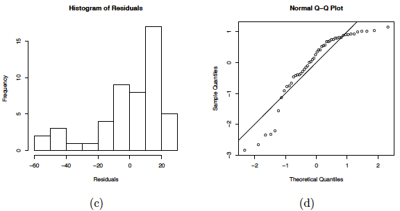
(c) Histogram of the residuals. (d) NPP for the Studentized residuals.
Residual plots of this linear regression analysis are also provided in the plot above. Notice in the residuals versus predictor plots how there is obvious curvature and it does not show uniform randomness as we have seen before. The histogram appears heavily left-skewed and does not show the ideal bell-shape for normality. Furthermore, the NPP seems to deviate from a straight line and curves down at the extreme percentiles. These plots alone suggest that there is something wrong with the model being used and indicate that a higher-order model may be needed.
The matrices for the second-degree polynomial model are:
\(\textbf{Y}=\left( \begin{array}{c} y_{1} \\ y_{2} \\ \vdots \\ y_{50} \\ \end{array} \right) \), \(\textbf{X}=\left( \begin{array}{cccc} 1 & x_{1} & x_{1}^{2} \\ 1 & x_{2} & x_{2}^{2} \\ \vdots & \vdots & \vdots \\ 1 & x_{50} & x_{50}^{2} \\ \end{array} \right)\), \(\vec{\beta}=\left( \begin{array}{c} \beta_{0} \\ \beta_{1} \\ \beta_{2} \\ \end{array} \right) \), \(\vec{\epsilon}=\left( \begin{array}{c} \epsilon_{1} \\ \epsilon_{2} \\ \vdots \\ \epsilon_{50} \\ \end{array} \right) \)
where the entries in Y and X would consist of the raw data. So as you can see, we are in a setting where the analysis techniques used in multiple linear regression (e.g., OLS) are applicable here.
Some general guidelines to keep in mind when estimating a polynomial regression model are:
- The fitted model is more reliable when it is built on a larger sample size n.
- Do not extrapolate beyond the limits of your observed values, particularly when the polynomial function has a pronounced curve such that an extraploation produces meaningless results beyond the scope of the model.
- Consider how large the size of the predictor(s) will be when incorporating higher degree terms as this may cause numerical overflow for the statistical software being used.
- Do not go strictly by low p-values to incorporate a higher degree term, but rather just use these to support your model only if the resulting residual plots looks reasonable. This is an example of a situation where you need to determine "practical significance" versus "statistical significance".
- In general, as is standard practice throughout regression modeling, your models should adhere to the hierarchy principle, which says that if your model includes \(X^{h}\) and \(X^{h}\) is shown to be a statistically significant predictor of Y, then your model should also include each \(X^{j}\) for all \(j<h\), whether or not the coefficients for these lower-order terms are significant.