Recall that data-based multicollinearity is multicollinearity that results from a poorly designed experiment, reliance on purely observational data, or the inability to manipulate the system on which the data are collected. We now know all the bad things that can happen in the presence of multicollinearity. And, we've learned how to detect multicollinearity. Now, let's learn how to reduce multicollinearity once we've discovered that it exists.
As the example in the previous section illustrated, one way of reducing data-based multicollinearity is to remove one or more of the violating predictors from the regression model. Another way is to collect additional data under different experimental or observational conditions. We'll investigate this alternative method in this section.
Before we do, let's quickly remind ourselves why we should care about reducing multicollinearity. It all comes down to drawing conclusions about the population slope parameters. If the variances of the estimated coefficients are inflated by multicollinearity, then our confidence intervals for the slope parameters are wider and therefore less useful. Eliminating or even reducing the multicollinearity, therefore, yields narrower, more useful confidence intervals for the slopes.
Example 12-3 Section
Researchers running the Allen Cognitive Level (ACL) Study were interested in the relationship of ACL test scores to the level of psychopathology. They, therefore, collected the following data on a set of 69 patients in a hospital psychiatry unit:
- Response \(y\) = ACL test score
- Predictor \(x_1\) = vocabulary (Vocab) score on the Shipley Institute of Living Scale
- Predictor \(x_2\) = abstraction (Abstract) score on the Shipley Institute of Living Scale
- Predictor \(x_3\) = score on the Symbol-Digit Modalities Test (SDMT)
For the sake of this example, I sampled 23 patients from the original data set in such a way as to ensure that a very high correlation exists between the two predictors Vocab and Abstract. A matrix plot of the resulting Allen Test n=23 data set:
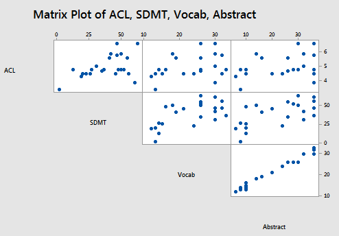
suggests that, indeed, a strong correlation exists between Vocab and Abstract. The correlations among the remaining pairs of predictors do not appear to be particularly strong.
Focusing only on the relationship between the two predictors Vocab and Abstract:
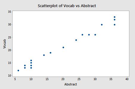
Pearson correlation of Vocab and Abstraction = 0.990
we do indeed see that a very strong relationship (r = 0.99) exists between the two predictors.
Let's see what havoc this high correlation wreaks on our regression analysis! Regressing the response y = ACL on the predictors SDMT, Vocab, and Abstract, we obtain:
Analysis of Variance
| Source | DF | Seq SS | Seq MS | F-Value | P-Value |
|---|---|---|---|---|---|
| Regression | 3 | 3.6854 | 1.22847 | 2.28 | 0.112 |
| SDMT | 1 | 3.6346 | 3.63465 | 6.74 | 0.018 |
| Vocab | 1 | 0.0406 | 0.04064 | 0.08 | 0.787 |
| Abstract | 1 | 0.0101 | 0.01014 | 0.02 | 0.892 |
| Error | 19 | 10.2476 | 0.53935 | ||
| Total | 22 | 13.9330 |
Modal Summary
| S | R-sq | R-sq(adj) | R-sq(pred) |
|---|---|---|---|
| 0.734404 | 26.45% | 14.84% | 0.00% |
Coefficients
| Term | Coef | SE Coef | T-Value | P-Value | VIF |
|---|---|---|---|---|---|
| Constant | 3.75 | 1.34 | 2.79 | 0.012 | |
| SDMT | 0.0233 | 0.0127 | 1.83 | 0.083 | 1.73 |
| Vocab | 0.028 | 0.152 | 0.19 | 0.855 | 49.29 |
| Abstract | -0.014 | 0.101 | -0.14 | 0.892 | 50.60 |
Yikes — the variance inflation factors for Vocab and Abstract are very large — 49.3 and 50.6, respectively!
What should we do about this? We could opt to remove one of the two predictors from the model. Alternatively, if we have a good scientific reason for needing both of the predictors to remain in the model, we could go out and collect more data. Let's try this second approach here.
For the sake of this example, let's imagine that we went out and collected more data, and in so doing, obtained the actual data collected on all 69 patients enrolled in the Allen Cognitive Level (ACL) Study. A matrix plot of the resulting Allen Test data set:
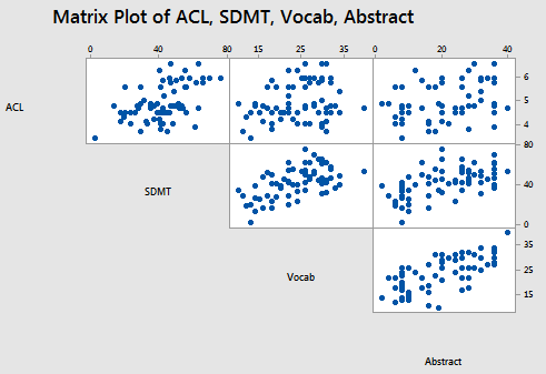
Pearson correlation of Vocab and Abstraction = 0.698
suggests that a correlation still exists between Vocab and Abstract — it is just a weaker correlation now.
Again, focusing only on the relationship between the two predictors Vocab and Abstract:
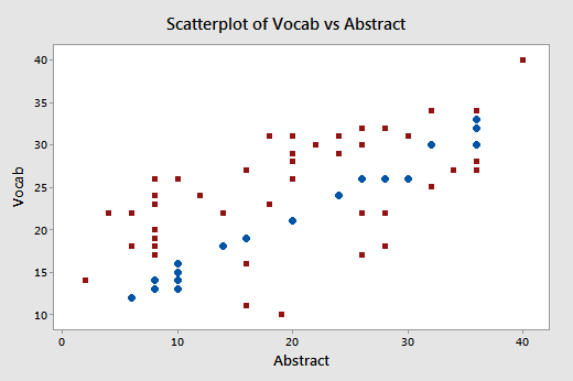
we do indeed see that the relationship between Abstract and Vocab is now much weaker (r = 0.698) than before. The round data points in blue represent the 23 data points in the original data set, while the square red data points represent the 46 newly collected data points. As you can see from the plot, collecting the additional data has expanded the "base" over which the "best fitting plane" will sit. The existence of this larger base allows less room for the plane to tilt from sample to sample, and thereby reduces the variance of the estimated slope coefficients.
Let's see if the addition of the new data helps to reduce the multicollinearity here. Regressing the response y = ACL on the predictors SDMT, Vocab, and Abstract:
Analysis of Variance
| Source | DF | Seq SS | Seq MS | F-Value | P-Value |
|---|---|---|---|---|---|
| Regression | 3 | 12.3009 | 4.1003 | 8.67 | 0.000 |
| SDMT | 1 | 11.6799 | 11.6799 | 24.69 | 0.000 |
| Vocab | 1 | 0.0979 | 0.0979 | 0.21 | 0.651 |
| Abstract | 1 | 0.5230 | 0.5230 | 1.11 | 0.297 |
| Error | 65 | 30.7487 | 0.4731 | ||
| Total | 68 | 43.0496 |
Modal Summary
| S | R-sq | R-sq(adj) | R-sq(pred) |
|---|---|---|---|
| 0.687791 | 28.57% | 25.28% | 19.93% |
Coefficients
| Term | Coef | SE Coef | T-Value | P-Value | VIF |
|---|---|---|---|---|---|
| Constant | 3.946 | 0.338 | 11.67 | 0.000 | |
| SDMT | 0.02740 | 0.00717 | 3.82 | 0.000 | 1.61 |
| Vocab | -0.0174 | 0.0181 | -0.96 | 0.339 | 2.09 |
| Abstract | 0.0122 | 0.0116 | 1.05 | 0.297 | 2.17 |
we find that the variance inflation factors are reduced significantly and satisfactorily. The researchers could now feel comfortable proceeding with drawing conclusions about the effects of the vocabulary and abstraction scores on the level of psychopathology.
Note! Section
One thing to keep in mind... In order to reduce the multicollinearity that exists, it is not sufficient to go out and just collect any ol' data. The data have to be collected in such a way as to ensure that the correlations among the violating predictors are actually reduced. That is, collecting more of the same kind of data won't help to reduce the multicollinearity. The data have to be collected to ensure that the "base" is sufficiently enlarged. Doing so, of course, changes the characteristics of the studied population, and therefore should be reported accordingly.