The General Linear F-Test Section
The "general linear F-test" involves three basic steps, namely:
- Define a larger full model. (By "larger," we mean one with more parameters.)
- Define a smaller reduced model. (By "smaller," we mean one with fewer parameters.)
- Use an F-statistic to decide whether or not to reject the smaller reduced model in favor of the larger full model.
As you can see by the wording of the third step, the null hypothesis always pertains to the reduced model, while the alternative hypothesis always pertains to the full model.
The easiest way to learn about the general linear test is to first go back to what we know, namely the simple linear regression model. Once we understand the general linear test for the simple case, we then see that it can be easily extended to the multiple-case model. We take that approach here.
The Full Model Section
The "full model", which is also sometimes referred to as the "unrestricted model," is the model thought to be most appropriate for the data. For simple linear regression, the full model is:
\(y_i=(\beta_0+\beta_1x_{i1})+\epsilon_i\)
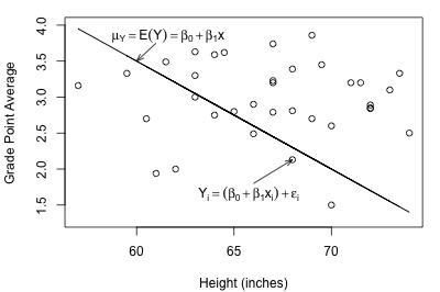
Here's a plot of a hypothesized full model for a set of data that we worked with previously in this course (student heights and grade point averages):
And, here's another plot of a hypothesized full model that we previously encountered (state latitudes and skin cancer mortalities):
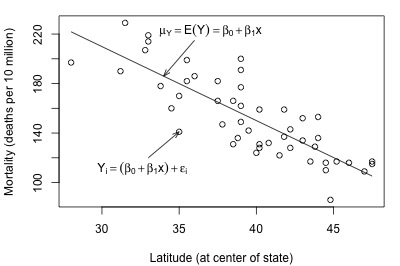
In each plot, the solid line represents what the hypothesized population regression line might look like for the full model. The question we have to answer in each case is "does the full model describe the data well?" Here, we might think that the full model does well in summarizing the trend in the second plot but not the first.
The Reduced Model Section
The "reduced model," which is sometimes also referred to as the "restricted model," is the model described by the null hypothesis \(H_{0}\). For simple linear regression, a common null hypothesis is \(H_{0} : \beta_{1} = 0\). In this case, the reduced model is obtained by "zeroing out" the slope \(\beta_{1}\) that appears in the full model. That is, the reduced model is:
\(y_i=\beta_0+\epsilon_i\)
This reduced model suggests that each response \(y_{i}\) is a function only of some overall mean, \(\beta_{0}\), and some error \(\epsilon_{i}\).
Let's take another look at the plot of student grade point average against height, but this time with a line representing what the hypothesized population regression line might look like for the reduced model:
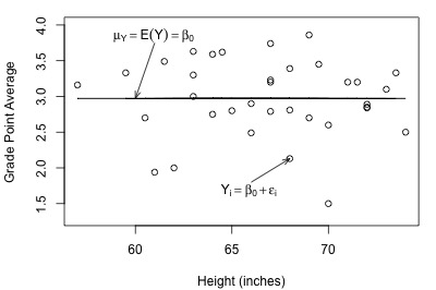
Not bad — there (fortunately?!) doesn't appear to be a relationship between height and grade point average. And, it appears as if the reduced model might be appropriate in describing the lack of a relationship between heights and grade point averages. What does the reduced model do for the skin cancer mortality example?
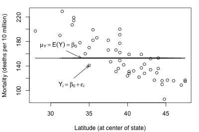
It doesn't appear as if the reduced model would do a very good job of summarizing the trend in the population.
F-Statistic Test Section
How do we decide if the reduced model or the full model does a better job of describing the trend in the data when it can't be determined by simply looking at a plot? What we need to do is to quantify how much error remains after fitting each of the two models to our data. That is, we take the general linear test approach:
- "Fit the full model" to the data.
- Obtain the least squares estimates of \(\beta_{0}\) and \(\beta_{1}\).
- Determine the error sum of squares, which we denote as "SSE(F)."
- "Fit the reduced model" to the data.
- Obtain the least squares estimate of \(\beta_{0}\).
- Determine the error sum of squares, which we denote as "SSE(R)."
Recall that, in general, the error sum of squares is obtained by summing the squared distances between the observed and fitted (estimated) responses:
\(\sum(\text{observed } - \text{ fitted})^2\)
Therefore, since \(y_i\) is the observed response and \(\hat{y}_i\) is the fitted response for the full model:
\(SSE(F)=\sum(y_i-\hat{y}_i)^2\)
And, since \(y_i\) is the observed response and \(\bar{y}\) is the fitted response for the reduced model:
\(SSE(R)=\sum(y_i-\bar{y})^2\)
Let's get a better feel for the general linear F-test approach by applying it to two different datasets. First, let's look at the Height and GPA data. The following plot of grade point averages against heights contains two estimated regression lines — the solid line is the estimated line for the full model, and the dashed line is the estimated line for the reduced model:
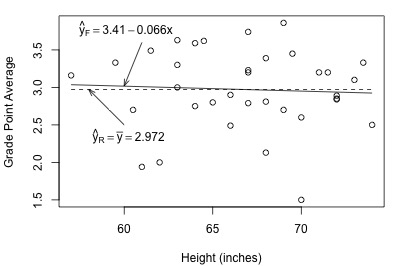
As you can see, the estimated lines are almost identical. Calculating the error sum of squares for each model, we obtain:
\(SSE(F)=\sum(y_i-\hat{y}_i)^2=9.7055\)
\(SSE(R)=\sum(y_i-\bar{y})^2=9.7331\)
The two quantities are almost identical. Adding height to the reduced model to obtain the full model reduces the amount of error by only 0.0276 (from 9.7331 to 9.7055). That is, adding height to the model does very little in reducing the variability in grade point averages. In this case, there appears to be no advantage in using the larger full model over the simpler reduced model.
Look what happens when we fit the full and reduced models to the skin cancer mortality and latitude dataset:
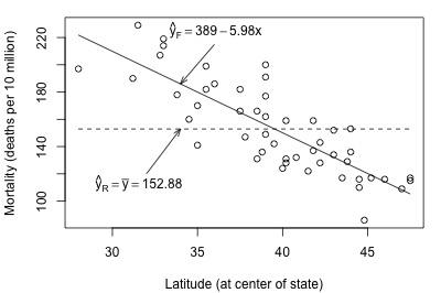
Here, there is quite a big difference between the estimated equation for the full model (solid line) and the estimated equation for the reduced model (dashed line). The error sums of squares quantify the substantial difference in the two estimated equations:
\(SSE(F)=\sum(y_i-\hat{y}_i)^2=17173\)
\(SSE(R)=\sum(y_i-\bar{y})^2=53637\)
Adding latitude to the reduced model to obtain the full model reduces the amount of error by 36464 (from 53637 to 17173). That is, adding latitude to the model substantially reduces the variability in skin cancer mortality. In this case, there appears to be a big advantage in using the larger full model over the simpler reduced model.
Where are we going with this general linear test approach? In short:
- The general linear test involves a comparison between SSE(R) and SSE(F).
- SSE(R) can never be smaller than SSE(F). It is always larger than (or possibly the same as) SSE(F).
- If SSE(F) is close to SSE(R), then the variation around the estimated full model regression function is almost as large as the variation around the estimated reduced model regression function. If that's the case, it makes sense to use the simpler reduced model.
- On the other hand, if SSE(F) and SSE(R) differ greatly, then the additional parameter(s) in the full model substantially reduce the variation around the estimated regression function. In this case, it makes sense to go with the larger full model.
How different does SSE(R) have to be from SSE(F) in order to justify using the larger full model? The general linear F-statistic:
\(F^*=\left( \dfrac{SSE(R)-SSE(F)}{df_R-df_F}\right)\div\left( \dfrac{SSE(F)}{df_F}\right)\)
helps answer this question. The F-statistic intuitively makes sense — it is a function of SSE(R)-SSE(F), the difference in the error between the two models. The degrees of freedom — denoted \(df_{R}\) and \(df_{F}\) — are those associated with the reduced and full model error sum of squares, respectively.
We use the general linear F-statistic to decide whether or not:
- to reject the null hypothesis \(H_{0}\colon\) The reduced model
- in favor of the alternative hypothesis \(H_{A}\colon\) The full model
In general, we reject \(H_{0}\) if F* is large — or equivalently if its associated P-value is small.
The test applied to the simple linear regression model Section
For simple linear regression, it turns out that the general linear F-test is just the same ANOVA F-test that we learned before. As noted earlier for the simple linear regression case, the full model is:
\(y_i=(\beta_0+\beta_1x_{i1})+\epsilon_i\)
and the reduced model is:
\(y_i=\beta_0+\epsilon_i\)
Therefore, the appropriate null and alternative hypotheses are specified either as:
- \(H_{0} \colon y_i = \beta_{0} + \epsilon_{i}\)
- \(H_{A} \colon y_i = \beta_{0} + \beta_{1} x_{i} + \epsilon_{i}\)
or as:
- \(H_{0} \colon \beta_{1} = 0 \)
- \(H_{A} \colon \beta_{1} ≠ 0 \)
The degrees of freedom associated with the error sum of squares for the reduced model is n-1, and:
\(SSE(R)=\sum(y_i-\bar{y})^2=SSTO\)
The degrees of freedom associated with the error sum of squares for the full model is n-2, and:
\(SSE(F)=\sum(y_i-\hat{y}_i)^2=SSE\)
Now, we can see how the general linear F-statistic just reduces algebraically to the ANOVA F-test that we know:
\(F^*=\left( \dfrac{SSE(R)-SSE(F)}{df_R-df_F}\right)\div\left( \dfrac{SSE(F)}{df_F}\right)\)
Can be rewritten by substituting...
\(\begin{aligned} &&df_{R} = n - 1\\ &&df_{F} = n - 2\\ &&SSE(R)=SSTO\\&&SSE(F)=SSE\end{aligned}\)
\(F^*=\left( \dfrac{SSTO-SSE}{(n-1)-(n-2)}\right)\div\left( \dfrac{SSE}{(n-2)}\right)=\frac{MSR}{MSE}\)
That is, the general linear F-statistic reduces to the ANOVA F-statistic:
\(F^*=\dfrac{MSR}{MSE}\)
For the student height and grade point average example:
\( F^*=\dfrac{MSR}{MSE}=\dfrac{0.0276/1}{9.7055/33}=\dfrac{0.0276}{0.2941}=0.094\)
For the skin cancer mortality example:
\( F^*=\dfrac{MSR}{MSE}=\dfrac{36464/1}{17173/47}=\dfrac{36464}{365.4}=99.8\)
The P-value is calculated as usual. The P-value answers the question: "what is the probability that we’d get an F* statistic as large as we did if the null hypothesis were true?" The P-value is determined by comparing F* to an F distribution with 1 numerator degree of freedom and n-2 denominator degrees of freedom. For the student height and grade point average example, the P-value is 0.761 (so we fail to reject \(H_{0}\) and we favor the reduced model), while for the skin cancer mortality example, the P-value is 0.000 (so we reject \(H_{0}\) and we favor the full model).
Example 6-2: Alcohol and muscle Strength Section
Does alcoholism have an effect on muscle strength? Some researchers (Urbano-Marquez, et al, 1989) who were interested in answering this question collected the following data (Alcohol Arm data) on a sample of 50 alcoholic men:
- x = the total lifetime dose of alcohol (kg per kg of body weight) consumed
- y = the strength of the deltoid muscle in the man's non-dominant arm
The full model is the model that would summarize a linear relationship between alcohol consumption and arm strength. The reduced model, on the other hand, is the model that claims there is no relationship between alcohol consumption and arm strength.
Therefore, the appropriate null and alternative hypotheses are specified either as:
- \(H_0 \colon y_i = \beta_0 + \epsilon_i \)
- \(H_A \colon y_i = \beta_0 + \beta_{1}x_i + \epsilon_i\)
or as:
- \(H_0 \colon \beta_1 = 0\)
- \(H_A \colon \beta_1 ≠ 0\)
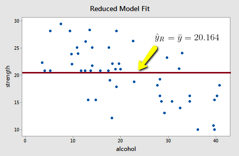
Upon fitting the reduced model to the data, we obtain:
and:
\(SSE(R)=\sum(y_i-\bar{y})^2=1224.32\)
Note that the reduced model does not appear to summarize the trend in the data very well.
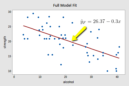
Upon fitting the full model to the data, we obtain:
and:
\(SSE(F)=\sum(y_i-\hat{y}_i)^2=720.27\)
The full model appears to describe the trend in the data better than the reduced model.
The good news is that in the simple linear regression case, we don't have to bother with calculating the general linear F-statistic. Minitab does it for us in the ANOVA table.
Click on the light bulb
Analysis of Variance
| Source | DF | Adj SS | Adj MS | F-Value | P-Value |
|---|---|---|---|---|---|
| Regression | 1 | 504.04 | 504.040 | 33.5899 | 0.000 |
| Error | 48 | 720.27 | 15.006 | ||
| Total | 49 | 1224.32 |
As you can see, Minitab calculates and reports both SSE(F) — the amount of error associated with the full model — and SSE(R) — the amount of error associated with the reduced model. The F-statistic is:
\( F^*=\dfrac{MSR}{MSE}=\dfrac{504.04/1}{720.27/48}=\dfrac{504.04}{15.006}=33.59\)
and its associated P-value is < 0.001 (so we reject \(H_{0}\) and favor the full model). We can conclude that there is a statistically significant linear association between lifetime alcohol consumption and arm strength.
This concludes our discussion of our first aside from the general linear F-test. Now, we move on to our second aside from sequential sums of squares.