Example 8-6: Additive Model Section
The Lesson8Ex1.txt dataset contains a response variable, Y, a quantitative predictor variable, X, and a categorical predictor variable, Cat, with three levels. We can code the information in Cat using two dummy indicator variables. A scatterplot of Y versus X with points marked by the level of Cat suggests three parallel regression lines with different intercepts but common slopes. We can confirm this with an F-test of the two X by dummy indicator variable interaction terms, which results in a high, non-significant p-value. We then refit without the interaction terms and confirm using individual t-tests that the intercept for level 2 differs from the intercept for level 1 and that the intercept for level 3 differs from the intercept for level 1.
Video Explanation
Example 8-7: Interaction Model Section
The Lesson8Ex2.txt dataset contains a response variable, Y, a quantitative predictor variable, X, and a categorical predictor variable, Cat, with three levels. We can code the information in Cat using two dummy indicator variables. A scatterplot of Y versus X with points marked by the level of Cat suggests three non-parallel regression lines with different intercepts and different slopes. We can confirm this with an F-test of the two X by dummy indicator variable interaction terms, which results in a low, significant p-value.
Video Explanation
Example 8-8: Muscle Mass Data Section
Suppose that we describe y = muscle mass as a function of \(x_1 = \text{ age and } x_2 = \text{ gender}\) for people in the 40 to 60 year-old age group. We could code the gender variable as \(x_2 = 1\) if the subject is female and \(x_2 = 0\) if the subject is male.
Consider the multiple regression equation
\(E\left(Y\right) = \beta_0 + \beta_1 x_1 + \beta_2 x_2\) .
The usual slope interpretation will work for \(\beta_2\), the coefficient that multiplies the gender indicator. Increasing gender by one unit simply moves us from male to female. Thus \(\beta_2\) = the difference between average muscle mass for females and males of the same age.
Example 8-9: Real Estate Air Conditioning Section
Consider the real estate dataset: Real estate data. Let us define
- \(Y =\) sale price of the home
- \(X_1 =\) square footage of home
- \(X_2 =\) whether the home has air conditioning or not.
To put the air conditioning variable into a model create a variable coded as either 1 or 0 to represent the presence or absence of air conditioning, respectively. With a 1, 0 coding for air conditioning and the model:
\(y_i = \beta_0 + \beta_1 x_{i,1} + \beta_2 x_{i,2} + \epsilon_i\)
the beta coefficient that multiplies the air conditioning variable will estimate the difference in average sale prices of homes that have air conditioning versus homes that do not, given that the homes have the same square foot area.
Suppose we think that the effect of air conditioning (yes or no) depends upon the size of the home. In other words, suppose that there is an interaction between the x-variables. To put an interaction into a model, we multiply the variables involved. The model here is
\(y_i = \beta_0 + \beta_1 x_{i,1} + \beta_2 x_{i,2} + \beta_3 x_{i,1}x_{i,2} + \epsilon_i\)
The data are from n = 521 homes. Statistical software output follows. Notice that there is a statistically significant result for the interaction term.
            Estimate Std. Error t value Pr(>|t|)
(Intercept)   -3.218     30.085  -0.107 0.914871
SqFeet       104.902     15.748   6.661 6.96e-11 ***
Air          -78.868     32.663  -2.415 0.016100 *
SqFeet.Air    55.888     16.580   3.371 0.000805 ***
The regression equation is:
Average SalePrice = −3.218 + 104.902 × SqrFeet − 78.868 × Air + 55.888 × SqrFeet × Air.
Suppose that a home has air conditioning. That means the variable Air = 1, so we’ll substitute Air = 1 in both places where Air occurs in the estimated model. This gives us
Average SalePrice = −3.218 + 104.902 × SqrFeet − 78.868(1) + 55.888 × SqrFeet × 1
= −82.086 + 160.790 × SqrFeet.
Suppose that a home does not have air conditioning. That means the variable Air = 0, so we’ll substitute Air = 0 in both places where Air occurs in the estimated model. This gives us
Average SalePrice = −3.218 + 104.902 × SqrFeet − 78.868(0) + 55.888 × SqrFeet × 0
= −3.218 + 104.902 × SqrFeet.
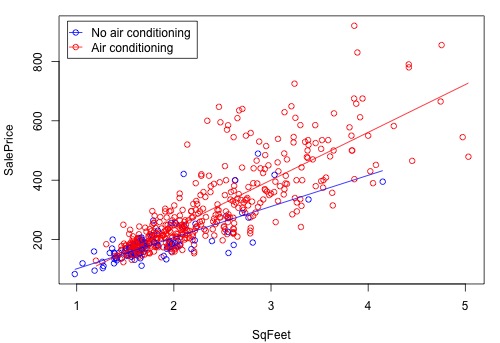
The figure below is a graph of the relationship between the sale price and square foot area for homes with air conditioning and homes without air conditioning. The equations of the two lines are the equations that we just derived above. The difference between the two lines increases as the square foot area increases. This means that the air conditioning versus no air conditioning difference in average sale price increases as the size of the home increases.
There is an increasing variance problem apparent in the above plot, which is even more obvious in the following residual plot:
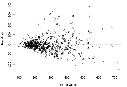
We'll return to this example in Section 9.3 to see how to remedy this.
Example 8-10: Hospital Infection Risk Data Section
Consider the hospital infection risk data: Infection Risk data. For this example, the data are limited to observations with an average length of stay ≤ 14 days, which reduces the overall sample size to n = 111. The variables we will analyze are the following:
\(Y =\) infection risk in hospital
\(X_1 =\) average length of patient’s stay (in days)
\(X_2 =\) a measure of the frequency of giving X-rays
\(X_3 =\) indication in which of 4 U.S. regions the hospital is located (northeast, north-central, south, west).
The focus of the analysis will be on regional differences. The region is a categorical variable so we must use indicator variables to incorporate region information into the model. There are four regions. The full set of indicator variables for the four regions is as follows:
\(I_1 = 1\) if hospital is in region 1 (north-east) and 0 if not
\(I_2 = 1\) if hospital is in region 2 (north-central) and 0 if not
\(I_3 = 1\) if hospital is in region 3 (south) and 0 if not
\(I_4 = 1\) if hospital is in region 4 (west), 0 otherwise.
To avoid a linear dependency in the X matrix, we will leave out one of these indicators when we form the model. Using all but the first indicator to describe regional differences (so that "north-east" is the reference region), a possible multiple regression model for \(E\left(Y\right)\), the mean infection risk, is:
\( E \left(Y\right) = \beta_0 + \beta_1 X_1 + \beta_2 X_2 + \beta_3 I_2 + \beta_4 I_3 + \beta_5 I_4\)
To understand the meanings of the beta coefficients, consider each region separately:
- For hospitals in region 1 (north-east), \(I_2 = 0, I_3 = 0, \text{ and } I_4 = 0 \), so
\begin{align} E \left(Y\right) &= \beta_0 + \beta_1 X_1 + \beta_2 X_2 + \beta_3 \left(0\right) + \beta_4 \left(0\right) +\beta_5 \left(0\right)\\
&= \beta_0 + \beta_1 X_1 + \beta_2 X_2 \end{align}
- For hospitals in region 2 (north-central), \(I_2 = 1 , I_3 = 0, \text{ and } I_4 = 0\), so
\begin{align} E \left(Y\right) &= \beta_0 + \beta_1 X_1 + \beta_2 X_2 + \beta_3 (1) + \beta_4 \left(0\right) +\beta_5 \left(0\right)\\
&= \beta_0 + \beta_1 X_1 + \beta_2 X_2 + \beta_3 \end{align}
- For hospitals in region 3 (south), \(I_2 = 0, I_3 = 1, \text{ and } I_4 = 0 \), so
\begin{align} E \left(Y\right) &= \beta_0 + \beta_1 X_1 + \beta_2 X_2 + \beta_3 \left(0\right) + \beta_4 (1) +\beta_5 \left(0\right)\\
&= \beta_0 + \beta_1 X_1 + \beta_2 X_2 + \beta_4\end{align}
- For hospitals in region 4 (west), \(I_2 = 0, I_3 = 0, \text{ and } I_4 = 1 \), so
\begin{align} E \left(Y\right) &= \beta_0 + \beta_1 X_1 + \beta_2 X_2 + \beta_3 \left(0\right) + \beta_4 \left(0\right) +\beta_5 (1)\\
&= \beta_0 + \beta_1 X_1 + \beta_2 X_2 + \beta_5\end{align}
A comparison of the four equations just given provides these interpretations of the coefficients that multiply indicator variables:
- \(\beta_3 =\) difference in mean infection risk for region 2 (north-central) versus region 1 (north-east), assuming the same values for stay \(\left(X_1\right)\) and X-rays \(\left(X_2\right)\)
- \(\beta_4 =\) difference in mean infection risk for region 3 (south) versus region 1 (north-east), assuming the same values for stay \(\left(X_1\right)\) and X-rays \(\left(X_2\right)\)
- \(\beta_5 =\) difference in mean infection risk for region 4 (west) versus region 1 (north-east), assuming the same values for stay \(\left(X_1\right)\) and X-rays \(\left(X_2\right)\)
Estimate Std. Error t value Pr(>|t|)
(Intercept) -2.134259   0.877347  -2.433  0.01668 *
Stay         0.505394   0.081455   6.205 1.11e-08 ***
Xray         0.017587   0.005649   3.113  0.00238 **
i2           0.171284   0.281475   0.609  0.54416
i3           0.095461   0.288852   0.330  0.74169
i4           1.057835   0.378077   2.798  0.00612 **
---
Signif. codes:  0 ‘***’ 0.001 ‘**’ 0.01 ‘*’ 0.05 ‘.’ 0.1 ‘ ’ 1
Residual standard error: 1.036 on 105 degrees of freedom
Multiple R-squared:  0.4198,	Adjusted R-squared:  0.3922
F-statistic: 15.19 on 5 and 105 DF,  p-value: 3.243e-11
Some interpretations of results for individual variables are:
- We have statistical significance for the sample coefficient that multiplies \( I_4 \left(\text{p-value} = 0.006\right)\). This is the sample coefficient that estimates the coefficient \(\beta_5\), so we have evidence of a difference in the infection risks for hospitals in region 4 (west) and hospitals in region 1 (north-east), assuming the same values for stay (X1) and X-rays (X2). The positive coefficient indicates that the infection risk is higher in the west.
- The non-significance for the coefficients multiplying \( I_2 \text{ and } I_3\) indicates no observed difference between mean infection risks in region 2 (north-central) versus region 1 (north-east) nor between region 3 (south) versus region 1 (north-east), assuming the same values for stay (X1) and X-rays (X2).
Next, the finding of a difference between mean infection risks in the northeast and west seems to be strong, but for the sake of an example, we’ll now consider an overall test of regional differences. There is, in fact, an argument for doing so beyond “for the sake of example.” To assess regional differences, we considered three significance tests (for the three indicator variables). When we carry out multiple inferences, the overall error rate is increased so we may be concerned about a “fluke” result for one of the comparisons. If there are no regional differences, we would not have any indicator variables for regions in the model.
- The null hypothesis that makes this happen is \(H_0 \colon \beta_3 = \beta_4 = \beta_5 = 0\).
- The reduced model is simply \(E \left(Y\right) = \beta_0 + \beta_1 X_1 + \beta_2 X_2 \). This model has SSE = 123.56 with error df = 108.
- The full model is \(E \left(Y\right) = \beta_0 + \beta_1 X_1 + \beta_2 X_2 + \beta_3 I_2 + \beta_4 I_3 + \beta_5 I_4\), the model that we have already estimated. This model has SSE = 112.71 with error df = 105.
The test statistic for \(H_0 \colon \beta_3 = \beta_4 = \beta_5 = 0\) is the general linear F-statistic calculated as
\(F=\dfrac{\frac{\text{SSE(reduced) - SSE(full)}}{\text{error df for reduced - error df for full}}}{\text{MSE(full)}}=\dfrac{\frac{123.56-112.71}{108-105}}{\frac{112.71}{105}}=3.369.\)
The degrees of freedom for this F-statistic are 3 and 105. We find that the probability of getting an F statistic as extreme or more extreme than 3.369 under an \(F_{3,105}\) distribution is 0.021 (i.e., the p-value). We reject the null hypothesis and conclude that at least one of \(\beta_3\), \(\beta_4 , \text{ and } \beta_5 \) is not 0. Our previous look at the tests for individual coefficients showed us that it is \(\beta_5 \) (measuring the difference between west and northeast) that we conclude is different from 0.
Finally, the results seem to indicate that the west is the only regional difference we see that has a higher infection risk than the other three regions. (If the north-central and south regions don’t differ from the northeast, it is reasonable to think that they don’t differ from each other as well.) We can test this by considering a reduced model in which the only region indicator is \( I_4 = 1\) if west, and 0 otherwise. The model is
\(E \left(Y\right) = \beta_0 + \beta_1 X_1 + \beta_2 X_2 + \beta_5 I_4\).
The null hypothesis leading to this reduced model is \(H_0 \colon \beta_3 = \beta_4 = 0\). This model has SSE = 113.11 with error df = 107.
The full model is still
\(E \left(Y\right) = \beta_0 + \beta_1X_1 + \beta_2X_2 + \beta_3 I_1 + \beta_4 I_2 + \beta_5 I_3\),
which has SSE = 112.71 with error df = 105. Finally,
\(F=\dfrac{\frac{\text{SSE(reduced) - SSE(full)}}{\text{error df for reduced - error df for full}}}{\text{MSE(full)}}=\dfrac{\frac{113.11-112.71}{107-105}}{\frac{112.71}{105}}=0.186.\)
The degrees of freedom for this F-statistic are 2 and 105. We find that the probability of getting an F-statistic as extreme or more extreme than 0.186 under an \(F_{2,105}\) distribution is 0.831 (i.e., the p-value). Thus, we cannot reject the null hypothesis and conclude that the west difference from the other three regions seems to be reasonable.