As stated in the lesson overview, multicollinearity exists whenever two or more of the predictors in a regression model are moderately or highly correlated. Now, you might be wondering why can't a researcher just collect his data in such a way to ensure that the predictors aren't highly correlated. Then, multicollinearity wouldn't be a problem, and we wouldn't have to bother with this silly lesson.
Unfortunately, researchers often can't control the predictors. Obvious examples include a person's gender, race, grade point average, math SAT score, IQ, and starting salary. For each of these predictor examples, the researcher just observes the values as they occur for the people in her random sample.
Multicollinearity happens more often than not in such observational studies. And, unfortunately, regression analyses most often take place on data obtained from observational studies. If you aren't convinced, consider the example data sets for this course. Most of the data sets were obtained from observational studies, not experiments. It is for this reason that we need to fully understand the impact of multicollinearity on our regression analyses.
Types of multicollinearity
- Structural multicollinearity is a mathematical artifact caused by creating new predictors from other predictors — such as creating the predictor \(x^{2}\) from the predictor x.
- Data-based multicollinearity, on the other hand, is a result of a poorly designed experiment, reliance on purely observational data, or the inability to manipulate the system on which the data are collected.
In the case of structural multicollinearity, the multicollinearity is induced by what you have done. Data-based multicollinearity is the more troublesome of the two types of multicollinearity. Unfortunately, it is the type we encounter most often!
Example 12-1 Section

Let's take a quick look at an example in which data-based multicollinearity exists. Some researchers observed — notice the choice of word! — the following Blood Pressure data on 20 individuals with high blood pressure:
- blood pressure (y = BP, in mm Hg)
- age (\(x_{1} = Age\), in years)
- weight (\(x_{2} = Weight\), in kg)
- body surface area (\(x_{3} = BSA\), in sq m)
- duration of hypertension (\(x_{4} = Dur\), in years)
- basal pulse (\(x_{5} = Pulse\), in beats per minute)
- stress index (\(x_{6} = Stress\))
The researchers were interested in determining if a relationship exists between blood pressure and age, weight, body surface area, duration, pulse rate, and/or stress level.
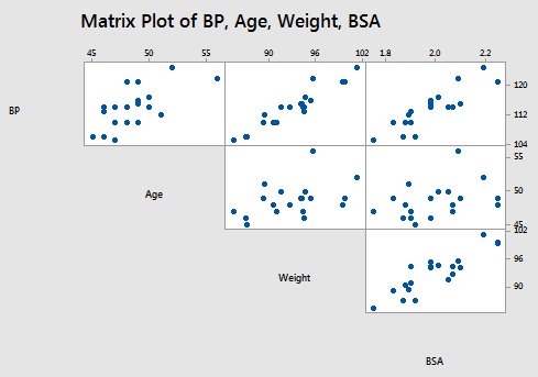
The matrix plot of BP, Age, Weight, and BSA:
and the matrix plot of BP, Dur, Pulse, and Stress:
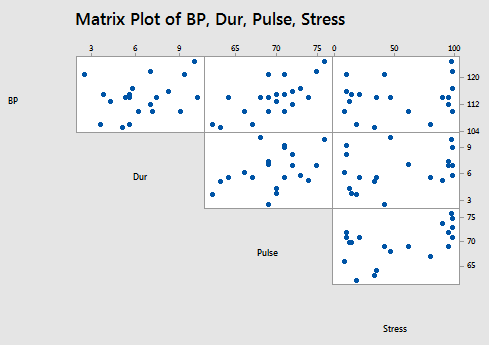
allow us to investigate the various marginal relationships between the response BP and the predictors. Blood pressure appears to be related fairly strongly to Weight and BSA, and hardly related at all to the Stress level.
The matrix plots also allow us to investigate whether or not relationships exist among the predictors. For example, Weight and BSA appear to be strongly related, while Stress and BSA appear to be hardly related at all.
The following correlation matrix:
Correlation: BP, Age, Weight, BSA, Dur, Pulse, Stress
| BP | Age | Weight | BSA | Dur | Pulse | |
|---|---|---|---|---|---|---|
| Age | 0.659 | |||||
| Weight | 0.950 | 0.407 | ||||
| BSA | 0.866 | 0.378 | 0.875 | |||
| Dur | 0.293 | 0.344 | 0.201 | 0.131 | ||
| Pulse | 0.721 | 0.619 | 0.659 | 0.465 | 0.402 | |
| Stress | 0.164 | 0.368 | 0.034 | 0.018 | 0.312 | 0.506 |
provides further evidence of the above claims. Blood pressure appears to be related fairly strongly to Weight (r = 0.950) and BSA (r = 0.866), and hardly related at all to Stress level (r = 0.164). And, Weight and BSA appear to be strongly related (r = 0.875), while Stress and BSA appear to be hardly related at all (r = 0.018). The high correlation among some of the predictors suggests that data-based multicollinearity exists.
Now, what we need to learn is the impact of multicollinearity on regression analysis. Let's go do it!