Example 8-4: Depression Treatments Section
Now that we've clarified what additive effects are, let's take a look at an example where including "interaction terms" is appropriate.
Some researchers (Daniel, 1999) were interested in comparing the effectiveness of three treatments for severe depression. For the sake of simplicity, we denote the three treatments A, B, and C. The researchers collected the following data (Depression Data) on a random sample of n = 36 severely depressed individuals:
- \(y_{i} =\) measure of the effectiveness of the treatment for individual i
- \(x_{i1} =\) age (in years) of individual i
- \(x_{i2} = 1\) if individual i received treatment A and 0, if not
- \(x_{i3} = 1\) if individual i received treatment B and 0, if not
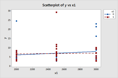
A scatter plot of the data with treatment effectiveness on the y-axis and age on the x-axis looks like this:
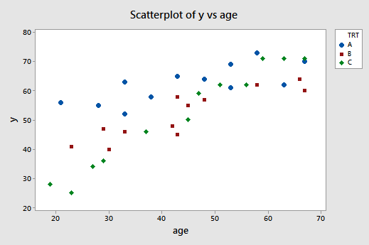
The blue circles represent the data for individuals receiving treatment A, the red squares represent the data for individuals receiving treatment B, and the green diamonds represent the data for individuals receiving treatment C.
In the previous example, the two estimated regression functions had the same slopes —that is, they were parallel. If you tried to draw three best-fitting lines through the data of this example, do you think the slopes of your lines would be the same? Probably not! In this case, we need to include what are called "interaction terms" in our formulated regression model.
A (second-order) multiple regression model with interaction terms is:
\(y_i=\beta_0+\beta_1x_{i1}+\beta_2x_{i2}+\beta_3x_{i3}+\beta_{12}x_{i1}x_{i2}+\beta_{13}x_{i1}x_{i3}+\epsilon_i\)
where:
- \(y_{i} =\) measure of the effectiveness of the treatment for individual i
- \(x_{i1} =\) age (in years) of individual i
- \(x_{i2} = 1\) if individual i received treatment A and 0, if not
- \(x_{i3} = 1\) if individual i received treatment B and 0, if not
and the independent error terms \(\epsilon_i\) follow a normal distribution with mean 0 and equal variance \(\sigma^{2}\). Perhaps not surprisingly, the terms \(x_{i} x_{i2}\) and \(x_{i1} x_{i3}\) are the interaction terms in the model.
Let's investigate our formulated model to discover in what way the predictors have an "interaction effect" on the response. We start by determining the formulated regression function for each of the three treatments. In short —after a little bit of algebra (see below) —we learn that the model defines three different regression functions —one for each of the three treatments:
| Treatment | Formulated regression function |
|---|---|
| If patient receives A, then \( \left(x_{i2} = 1, x_{i3} = 0 \right) \) and ... |
\(\mu_Y=(\beta_0+\beta_2)+(\beta_1+\beta_{12})x_{i1}\) |
| If patient receives B, then \( \left(x_{i2} = 0, x_{i3} = 1 \right) \) and ... |
\(\mu_Y=(\beta_0+\beta_3)+(\beta_1+\beta_{13})x_{i1}\) |
| If patient receives C, then \( \left(x_{i2} = 0, x_{i3} = 0 \right) \) and ... |
\(\mu_Y=\beta_0+\beta_{1}x_{i1}\) |
So, in what way does including the interaction terms, \(x_{i1} x_{i2}\) and \(x_{i1} x_{i3}\), in the model imply that the predictors have an "interaction effect" on the mean response? Note that the slopes of the three regression functions differ —the slope of the first line is \(\beta_1 + \beta_{12}\), the slope of the second line is \(\beta_1 + \beta_{13}\), and the slope of the third line is \(\beta_1\). What does this mean in a practical sense? It means that...
- the effect of the individual's age \(\left( x_1 \right)\) on the treatment's mean effectiveness \(\left(\mu_Y \right)\) depends on the treatment \(\left(x_2 \text{ and } x_3\right)\), and ...
- the effect of treatment \(\left(x_2 \text{ and } x_3\right)\) on the treatment's mean effectiveness \(\left(\mu_Y \right)\) depends on the individual's age \(\left( x_1 \right)\).
In general, then, what does it mean for two predictors "to interact"?
- Two predictors interact if the effect on the response variable of one predictor depends on the value of the other.
- A slope parameter can no longer be interpreted as the change in the mean response for each unit increase in the predictor, while the other predictors are held constant.
And, what are "interaction effects"?
A regression model contains interaction effects if the response function is not additive and cannot be written as a sum of functions of the predictor variables. That is, a regression model contains interaction effects if:
\(\mu_Y \ne f_1(x_1)+f_1(x_1)+ \cdots +f_{p-1}(x_{p-1})\)
For our example concerning treatment for depression, the mean response:
\(\mu_Y=\beta_0+\beta_1x_{1}+\beta_2x_{2}+\beta_3x_{3}+\beta_{12}x_{1}x_{2}+\beta_{13}x_{1}x_{3}\)
can not be separated into distinct functions of each of the individual predictors. That is, there is no way of "breaking apart" \(\beta_{12} x_1 x_2 \text{ and } \beta_{13} x_1 x_3\) into distinct pieces. Therefore, we say that \(x_1 \text{ and } x_2\) interact, and \(x_1 \text{ and } x_3\) interact.
In returning to our example, let's recall that the appropriate steps in any regression analysis are:
- Model building
- Model formulation
- Model estimation
- Model evaluation
- Model use
So far, within the model-building step, all we've done is formulate the regression model as:
\(y_i=\beta_0+\beta_1x_{i1}+\beta_2x_{i2}+\beta_3x_{i3}+\beta_{12}x_{i1}x_{i2}+\beta_{13}x_{i1}x_{i3}+\epsilon_i\)
We can use Minitab —or any other statistical software for that matter —to estimate the model. Doing so, Minitab reports:
Regression Equation
y = 6.21 + 1.0334 age + 41.30 x2+ 22.71 x3 - 0.703 agex2 - 0.510 agex3
Now, if we plug the possible values for \(x_2 \text{ and } x_3\) into the estimated regression function, we obtain the three "best fitting" lines —one for each treatment (A, B, and C) —through the data. Here's the algebra for determining the estimated regression function for patients receiving treatment A.
Doing similar algebra for patients receiving treatments B and C, we obtain:
| Treatment | Estimated regression function |
|---|---|
| If patient receives A, then \(\left(x_2 = 1, x_3 = 0 \right)\) and ... |
\(\hat{y}=47.5+0.33x_1\) |
| If patient receives B, then \(\left(x_2 = 0, x_3 = 1 \right)\) and ... |
\(\hat{y}=28.9+0.52x_1\) |
| If patient receives C, then \(\left(x_2 = 0, x_3 = 0 \right)\) and ... |
\(\hat{y}=6.21+1.03x_1\) |
And, plotting the three "best fitting" lines, we obtain:
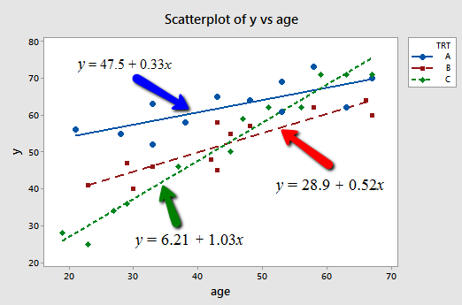
What do the estimated slopes tell us?
- For patients in this study receiving treatment A, the effectiveness of the treatment is predicted to increase by 0.33 units for every additional year in age.
- For patients in this study receiving treatment B, the effectiveness of the treatment is predicted to increase by 0.52 units for every additional year in age.
- For patients in this study receiving treatment C, the effectiveness of the treatment is predicted to increase by 1.03 units for every additional year in age.
In short, the effect of age on the predicted treatment effectiveness depends on the treatment given. That is, age appears to interact with treatment in its impact on treatment effectiveness. The interaction is exhibited graphically by the "nonparallelness" (is that a word?) of the lines.
Of course, our primary goal is not to draw conclusions about this particular sample of depressed individuals, but rather about the entire population of depressed individuals. That is, we want to use our estimated model to draw conclusions about the larger population of depressed individuals. Before we do so, however, we first should evaluate the model.
The residuals versus fits plot:
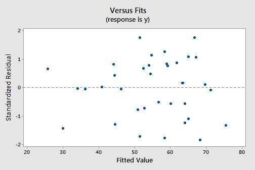
exhibits all of the "good" behavior, suggesting that the model fits well, there are no obvious outliers, and the error variances are indeed constant. And, the normal probability plot:
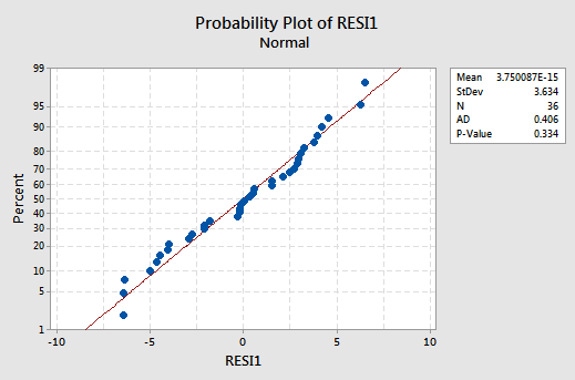
exhibits a linear trend and a large P-value, suggesting that the error terms are indeed normally distributed.
Having successfully built —formulated, estimated, and evaluated —a model, we now can use the model to answer our research questions. Let's consider two different questions that we might want to be answered.
First research question. For every age, is there a difference in the mean effectiveness for the three treatments? As is usually the case, our formulated regression model helps determine how to answer the research question. Our formulated regression model suggests that answering the question involves testing whether the population regression functions are identical.
That is, we need to test the null hypothesis \(H_0 \colon \beta_2 = \beta_3 =\beta_{12} = \beta_{13} = 0\) against the alternative \(H_A \colon\) at least one of these slope parameters is not 0.
We know how to do that! The relevant software output:
Analysis of Variance
| Source | DF | Seq SS | Seq MS | F-Value | P-Value |
|---|---|---|---|---|---|
| Regression | 5 | 4932.85 | 986.57 | 64.04 | 0.000 |
| age | 5 | 3424.43 | 3424.43 | 222.29 | 0.000 |
| x2 | 1 | 803.80 | 803.80 | 52.18 | 0.000 |
| x3 | 1 | 1.19 | 1.19 | 0.08 | 0.783 |
| agex2 | 1 | 375.00 | 375.00 | 24.34 | 0.000 |
| agex3 | 1 | 328.42 | 328.42 | 21.32 | 0.000 |
| Error | 30 | 462.15 | 15.40 | ||
| Lack-of-Fit | 27 | 285.15 | 10.56 | 0.18 | 0.996 |
| Pure Error | 3 | 177.00 | 59.00 | ||
| Total | 35 | 5395.0 |
tells us that the appropriate partial F-statistic for testing the above hypothesis is:
\(F=\frac{(803.8+1.19+375+328.42)/4}{15.4}=24.49\)
And, Minitab tells us:
F Distribution with 4 DF in Numerator and 30 DF in denominator
| x | \(p(X \leq x)\) |
|---|---|
| 24.49 | 1.00000 |
that the probability of observing an F-statistic —with 4 numerator and 30 denominator degrees of freedom —less than our observed test statistic 24.49 is > 0.999. Therefore, our P-value is < 0.001. We can reject our null hypothesis. There is sufficient evidence at the \(\alpha = 0.05\) level to conclude that there is a significant difference in the mean effectiveness for the three treatments.
Second research question. Does the effect of age on the treatment's effectiveness depend on the treatment? Our formulated regression model suggests that answering the question involves testing whether the two interaction parameters \(\beta_{12} \text{ and } \beta_{13}\) are significant. That is, we need to test the null hypothesis \(H_0 \colon \beta_{12} = \beta_{13} = 0\) against the alternative \(H_A \colon\) at least one of the interaction parameters is not 0.
The relevant software output:
Analysis of Variance
| Source | DF | Seq SS | Seq MS | F-Value | P-Value |
|---|---|---|---|---|---|
| Regression | 5 | 4932.85 | 986.57 | 64.04 | 0.000 |
| age | 5 | 3424.43 | 3424.43 | 222.29 | 0.000 |
| x2 | 1 | 803.80 | 803.80 | 52.18 | 0.000 |
| x3 | 1 | 1.19 | 1.19 | 0.08 | 0.783 |
| agex2 | 1 | 375.00 | 375.00 | 24.34 | 0.000 |
| agex3 | 1 | 328.42 | 328.42 | 21.32 | 0.000 |
| Error | 30 | 462.15 | 15.40 | ||
| Lack-of-Fit | 27 | 285.15 | 10.56 | 0.18 | 0.996 |
| Pure Error | 3 | 177.00 | 59.00 | ||
| Total | 35 | 5395.0 |
tells us that the appropriate partial F-statistic for testing the above hypothesis is:
\(F=\dfrac{(375+328.42)/2}{15.4}=22.84\)
And, Minitab tells us:
F Distribution with 2 DF in Numerator and 30 DF in denominator
| x | \(p(X \leq x)\) |
|---|---|
| 22.84 | 1.00000 |
that the probability of observing an F-statistic — with 2 numerator and 30 denominator degrees of freedom — less than our observed test statistic 22.84 is > 0.999. Therefore, our P-value is < 0.001. We can reject our null hypothesis. There is sufficient evidence at the \(\alpha = 0.05\) level to conclude that the effect of age on the treatment's effectiveness depends on the treatment.
Try It!
A model with an interaction term Section
-
For the depression study, plug the appropriate values for \(x_2 \text{ and } x_3\) into the formulated regression function and perform the necessary algebra to determine:
- The formulated regression function for patients receiving treatment B.
- The formulated regression function for patients receiving treatment C.
\(\mu_Y = \beta_0+\beta_1x1+\beta_2 x_2+\beta_3 x_3+\beta_{12}x_1 x_2+\beta_{13} x_1 x_3\)
\(\mu_Y = \beta_0+\beta_1 x_1+\beta_2(0)+\beta_3(1)+\beta_{12} x_1(0)+\beta_{13} x_1(1) = (\beta_0+\beta_3)+(\beta_1+\beta_{13})x_1\)
\(\mu_Y = \beta_0+\beta_1 x_1+\beta_2(0)+\beta_3(0)+\beta_{12} x_1(0)+\beta_{13} x_1(0) = \beta_0+\beta_1 x_1\)
-
Treatment B, \(x_2 = 0 , x_3 = 1\), so
-
Treatment C, \(x_2 = 0 , x_3 = 0\), so
-
For the depression study, plug the appropriate values for \(x_2 \text{ and } x_3\) into the estimated regression function and perform the necessary algebra to determine:
- The estimated regression function for patients receiving treatment B.
- The estimated regression function for patients receiving treatment C.
\(\hat{y} = 6.21 + 1.0334 x_1 + 41.30 x_2+22.71 x_3 - 0.703 x_1 x_2 - 0.510 x_1 x_3\)
\(\hat{y} = 6.21 + 1.0334 x_1 + 41.30(0) + 22.71(1) - 0.703 x_1(0) - 0.510 x_1(1) = (6.21 + 22.71)+(1.0334 - 0.510) x_1 = 28.92 + 0.523 x_1\)
\(\hat{y} = 6.21 + 1.0334 x_1 + 41.30(0) + 22.71(0) - 0.703 x_1(0) - 0.510 x_1(0) = 6.21 + 1.033 x_1\)
-
Treatment B, \(x_2 = 0 , x_3 = 1\), so
-
Treatment C, \(x_2 = 0 , x_3 = 0\), so
-
For the first research question that we addressed for the depression study, show that there is no difference in the mean effectiveness between treatments B and C, for all ages, provided that \(\beta_3 = 0 \text{ and } \beta_{13} = 0\). (HINT: Follow the argument presented in the chalk-talk comparing treatments A and C.)
\(\mu_Y|\text{Treatment B} - \mu_Y|\text{Treatment C} = (\beta_0 + \beta_3)+(\beta_1 + \beta_{13}) x_1 - (\beta_0 + \beta_1 x_1) = \beta_3 + \beta_{13} x_1 = 0\), if \(\beta_3 = \beta_{13} = 0\)
-
A study of atmospheric pollution on the slopes of the Blue Ridge Mountains (Tennessee) was conducted. The Lead Moss data contains the levels of lead found in 70 fern moss specimens (in micrograms of lead per gram of moss tissue) collected from the mountain slopes, as well as the elevation of the moss specimen (in feet) and the direction (1 if east, 0 if west) of the slope face.
- Write the equation of a second-order model relating mean lead level, E(y), to elevation \(\left(x_1 \right)\) and the slope face \(\left(x_2 \right)\) that includes an interaction between elevation and slope face in the model.
- Graph the relationship between mean lead level and elevation for the different slope faces that are hypothesized by the model in part a.
- In terms of the β's of the model in part a, give the change in lead level for every one-foot increase in elevation for moss specimens on the east slope.
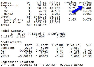
- Fit the model in part a to the data using an available statistical software package. Is the overall model statistically useful for predicting lead level? Test using \(α = 0.10\).
- Write the estimated equation of the model in part a relating mean lead level, E(y), to elevation \(\left(x_1 \right)\) and slope face \(\left(x_2 \right)\).
Since the p-value for testing whether the overall model is statistically useful for predicting lead level is 0.857, we conclude that this model is not statistically useful.
(e) The estimated equation is shown in the Minitab output above, but since the model is not statistically useful, this equation doesn’t do us much good.
-
\(\mu_Y = \beta_0 + \beta_1 x_1 + \beta_2 x_2 + \beta_{12} x_1 x_2\)
-
-
East slope, \(x_2=1\), \(\mu_Y = \beta_0 + \beta_1 x_1 + \beta_2(1) + \beta_{12} x_1(1) = (\beta_0 + \beta_2)+(\beta_1 + \beta_{12}) x_1\), so average lead level changes by \(\beta_1 + \beta_{12}\) micrograms of lead per gram of moss tissue for every one foot increase in elevation for moss specimens on the east slope.
-