We have worked hard to come up with formulas for the intercept \(b_{0}\) and the slope \(b_{1}\) of the least squares regression line. But, we haven't yet discussed what \(b_{0}\) and \(b_{1}\) estimate.
What do \(b_{0}\) and \(b_{1}\) estimate?
Let's investigate this question with another example. Below is a plot illustrating a potential relationship between the predictor "high school grade point average (GPA)" and the response "college entrance test score." Only five groups ("subpopulations") of students are considered — those with a GPA of 1, those with a GPA of 2, ..., and those with a GPA of 4.
Let's focus for now just on those students who have a GPA of 1. As you can see, there are so many data points — each representing one student — that the data points run together. That is, the data on the entire subpopulation of students with a GPA of 1 are plotted. And, similarly, the data on the entire subpopulation of students with GPAs of 2, 3, and 4 are plotted.
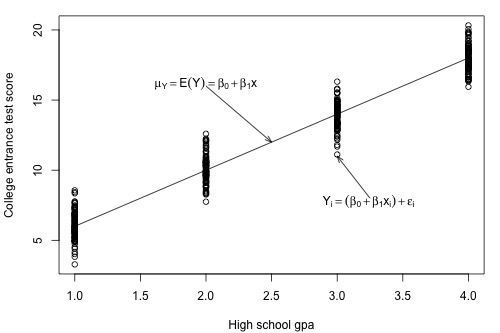
Now, take the average college entrance test score for students with a GPA of 1. And, similarly, take the average college entrance test score for students with a GPA of 2, 3, and 4. Connecting the dots — that is, the averages — you get a line, which we summarize by the formula \(\mu_Y=\mbox{E}(Y)=\beta_0 + \beta_1x\). The line — which is called the "population regression line" — summarizes the trend in the population between the predictor x and the mean of the responses \(\mu_{Y}\). We can also express the average college entrance test score for the \(i^{th}\) student, \(\mbox{E}(Y_i)=\beta_0 + \beta_1x_i\). Of course, not every student's college entrance test score will equal the average \(\mbox{E}(Y_i)\). There will be some errors. That is, any student's response \(y_{i}\) will be the linear trend \(\beta_0 + \beta_1x_i\) plus some error \(\epsilon_i\). So, another way to write the simple linear regression model is \(y_i = \mbox{E}(Y_i) + \epsilon_i = \beta_0 + \beta_1x_i + \epsilon_i\).
When looking to summarize the relationship between a predictor x and a response y, we are interested in knowing the population regression line \(\mu_Y=\mbox{E}(Y)=\beta_0 + \beta_1x\). The only way we could ever know it, though, is to be able to collect data on everybody in the population — most often an impossible task. We have to rely on taking and using a sample of data from the population to estimate the population regression line.
Let's take a sample of three students from each of the subpopulations — that is, three students with a GPA of 1, three students with a GPA of 2, ..., and three students with a GPA of 4 — for a total of 12 students. As the plot below suggests, the least squares regression line \(\hat{y}=b_0+b_1x\) through the sample of 12 data points estimates the population regression line \(\mu_Y=E(Y)=\beta_0 + \beta_1x\). That is, the sample intercept \(b_{0}\) estimates the population intercept \( \beta_{0}\) and the sample slope \(b_{1}\) estimates the population slope \( \beta_{1}\).
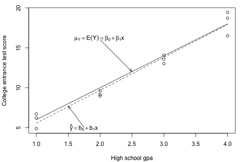
The least squares regression line doesn't match the population regression line perfectly, but it is a pretty good estimate. And, of course, we'd get a different least squares regression line if we took another (different) sample of 12 such students. Ultimately, we are going to want to use the sample slope \(b_{1}\) to learn about the parameter we care about, the population slope \( \beta_{1}\). And, we will use the sample intercept \(b_{0}\) to learn about the population intercept \(\beta_{0}\).
In order to draw any conclusions about the population parameters \( \beta_{0}\) and \( \beta_{1}\), we have to make a few more assumptions about the behavior of the data in a regression setting. We can get a pretty good feel for the assumptions by looking at our plot of GPA against college entrance test scores.
First, notice that when we connected the averages of the college entrance test scores for each of the subpopulations, it formed a line. Most often, we will not have the population of data at our disposal as we pretend to do here. If we didn't, do you think it would be reasonable to assume that the mean college entrance test scores are linearly related to high school grade point averages?
Again, let's focus on just one subpopulation, those students who have a GPA of 1, say. Notice that most of the college entrance scores for these students are clustered near the mean of 6, but a few students did much better than the subpopulation's average scoring around a 9, and a few students did a bit worse scoring about a 3. Do you get the picture? Thinking instead about the errors, \(\epsilon_i\), most of the errors for these students are clustered near the mean of 0, but a few are as high as 3 and a few are as low as -3. If you could draw a probability curve for the errors above this subpopulation of data, what kind of a curve do you think it would be? Does it seem reasonable to assume that the errors for each subpopulation are normally distributed?
Looking at the plot again, notice that the spread of the college entrance test scores for students whose GPA is 1 is similar to the spread of the college entrance test scores for students whose GPA is 2, 3, and 4. Similarly, the spread of the errors is similar, no matter the GPA. Does it seem reasonable to assume that the errors for each subpopulation have equal variance?
Does it also seem reasonable to assume that the error for one student's college entrance test score is independent of the error for another student's college entrance test score? I'm sure you can come up with some scenarios — cheating students, for example — for which this assumption would not hold, but if you take a random sample from the population, it should be an assumption that is easily met.
We are now ready to summarize the four conditions that comprise "the simple linear regression model:"
- Linear Function: The mean of the response, \(\mbox{E}(Y_i)\), at each value of the predictor, \(x_i\), is a Linear function of the \(x_i\).
- Independent: The errors, \( \epsilon_{i}\), are Independent.
- Normally Distributed: The errors, \( \epsilon_{i}\), at each value of the predictor, \(x_i\), are Normally distributed.
- Equal variances (denoted \(\sigma^{2}\)): The errors, \( \epsilon_{i}\), at each value of the predictor, \(x_i\), have Equal variances (denoted \(\sigma^{2}\)).
Do you notice what the first highlighted letters spell? " LINE." And, what are we studying in this course? Lines! Get it? You might find this mnemonic a useful way to remember the four conditions that make up what we call the "simple linear regression model." Whenever you hear "simple linear regression model," think of these four conditions!
An equivalent way to think of the first (linearity) condition is that the mean of the error, \(\mbox{E}(\epsilon_i)\), at each value of the predictor, \(x_i\), is zero. An alternative way to describe all four assumptions is that the errors, \(\epsilon_i\), are independent normal random variables with mean zero and constant variance, \(\sigma^2\).