In this section, we learn the distinction between outliers and high-leverage observations. In short:
- An outlier is a data point whose response y does not follow the general trend of the rest of the data.
- A data point has high leverage if it has "extreme" predictor x values. With a single predictor, an extreme x value is simply one that is particularly high or low. With multiple predictors, extreme x values may be particularly high or low for one or more predictors or may be "unusual" combinations of predictor values (e.g., with two predictors that are positively correlated, an unusual combination of predictor values might be a high value of one predictor paired with a low value of the other predictor).
Note that — for our purposes — we consider a data point to be an outlier only if it is extreme with respect to the other y values, not the x values.
A data point is influential if it unduly influences any part of regression analysis, such as the predicted responses, the estimated slope coefficients, or the hypothesis test results. Outliers and high-leverage data points have the potential to be influential, but we generally have to investigate further to determine whether or not they are actually influential.
One advantage of the case in which we have only one predictor is that we can look at simple scatter plots in order to identify any outliers and influential data points. Let's take a look at a few examples that should help to clarify the distinction between the two types of extreme values.
Example 11-1 Section
Based on the definitions above, do you think the following influence1 data set contains any outliers? Or, any high-leverage data points?
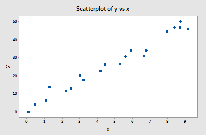
You got it! All of the data points follow the general trend of the rest of the data, so there are no outliers (in the y direction). And, none of the data points are extreme with respect to x, so there are no high leverage points. Overall, none of the data points would appear to be influential with respect to the location of the best-fitting line.
Example 11-2 Section
Now, how about this example? Do you think the following influence2 data set contains any outliers? Or, any high-leverage data points?
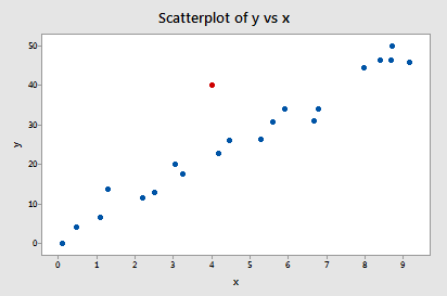
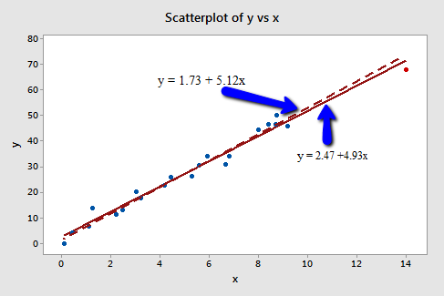
Of course! Because the red data point does not follow the general trend of the rest of the data, it would be considered an outlier. However, this point does not have an extreme x value, so it does not have high leverage. Is the red data point influential? An easy way to determine if the data point is influential is to find the best-fitting line twice — once with the red data point included and once with the red data point excluded. The following plot illustrates the two best-fitting lines:
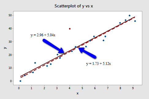
Wow — it's hard to even tell the two estimated regression equations apart! The solid line represents the estimated regression equation with the red data point included, while the dashed line represents the estimated regression equation with the red data point taken excluded. The slopes of the two lines are very similar — 5.04 and 5.12, respectively.
Do the two samples yield different results when testing \(H_0 \colon \beta_1 = 0\)? Well, we obtain the following output when the red data point is included:
Model Summary
| S | R-sq | R-sq(adj) | R-sq(pred) |
|---|---|---|---|
| 4.71075 | 91.01% | 90.53% | 89.61% |
Model Summary
| Term | Coef | SE Coef | T-Value | P-Value | VIF |
|---|---|---|---|---|---|
| Constant | 2.96 | 2.01 | 1.47 | 0.157 | |
| X | 5.037 | 0.363 | 13.86 | 0.000 | 1.00 |
Regression Equation
\(\widehat{y} = 2.96 + 5.037 x\)
and the following output when the red data point is excluded:
Model Summary
| S | R-sq | R-sq(adj) | R-sq(pred) |
|---|---|---|---|
| 2.59199 | 97.32% | 97.17% | 96.63% |
Model Summary
| Term | Coef | SE Coef | T-Value | P-Value | VIF |
|---|---|---|---|---|---|
| Constant | 1.73 | 1.12 | 1.55 | 0.140 | |
| X | 5.117 | 0.200 | 25.55 | 0.000 | 1.00 |
Regression Equation
\(\widehat{y} = 1.73 + 5.117 x\)
There certainly are some minor side effects of including the red data point, but none too serious:
- The \(R^{2}\) value has decreased slightly, but the relationship between y and x would still be deemed strong.
- The standard error of \(b_1\), which is used in calculating our confidence interval for \(\beta_1\), is larger when the red data point is included, thereby increasing the width of our confidence interval. You may recall that the standard error of \(b_1\) depends on the mean squared error MSE, which quantifies the difference between the observed and predicted responses. It is because the red data point is an outlier — in the y direction — that the standard error of \(b_1\) increases, not because the data point is influential in any way.
- In each case, the P-value for testing \(H_0 \colon \beta_1 = 0\) is less than 0.001. In either case, we can conclude that there is sufficient evidence at the 0.05 level to conclude that, in the population, x is related to y.
In short, the predicted responses, estimated slope coefficients, and hypothesis test results are not affected by the inclusion of the red data point. Therefore, the data point is not deemed influential. In summary, the red data point is not influential and does not have high leverage, but it is an outlier.
Example 11-3: Section
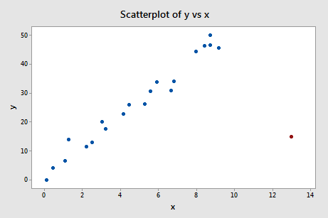
Now, how about this example? Do you think the following influence3 data set contains any outliers? Or, any high-leverage data points?
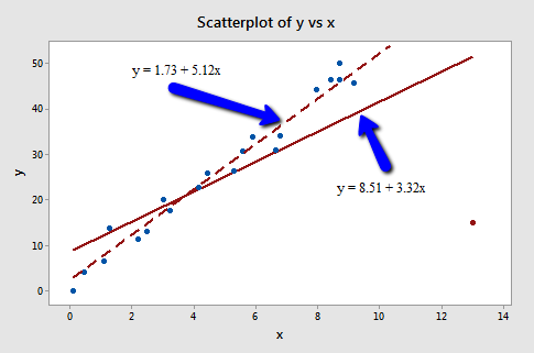
In this case, the red data point does follow the general trend of the rest of the data. Therefore, it is not deemed an outlier here. However, this point does have an extreme x value, so it does have high leverage. Is the red data point influential? It certainly appears to be far removed from the rest of the data (in the x direction), but is that sufficient to make the data point influential in this case?
The following plot illustrates two best-fitting lines — one obtained when the red data point is included and one obtained when the red data point is excluded:
Again, it's hard to even tell the two estimated regression equations apart! The solid line represents the estimated regression equation with the red data point included, while the dashed line represents the estimated regression equation with the red data point taken excluded. The slopes of the two lines are very similar — 4.927 and 5.117, respectively.
Do the two samples yield different results when testing \(H_0 \colon \beta_1 = 0\)? Well, we obtain the following output when the red data point is included:
Model Summary
| S | R-sq | R-sq(adj) | R-sq(pred) |
|---|---|---|---|
| 2.70911 | 97.74% | 97.62% | 97.04% |
Model Summary
| Term | Coef | SE Coef | T-Value | P-Value | VIF |
|---|---|---|---|---|---|
| Constant | 2.47 | 1.08 | 2.29 | 0.033 | |
| x | 4.927 | 0.172 | 28.66 | 0.000 | 1.00 |
Regression Equation
\(\widehat{y} = 2.47 + 4927 x\)
and the following output when the red data point is excluded:
Model Summary
| S | R-sq | R-sq(adj) | R-sq(pred) |
|---|---|---|---|
| 2.59199 | 97.32% | 97.17% | 96.63% |
Model Summary
| Term | Coef | SE Coef | T-Value | P-Value | VIF |
|---|---|---|---|---|---|
| Constant | 1.73 | 1.12 | 1.55 | 0.140 | |
| x | 5.117 | 0.200 | 25.55 | 0.000 | 1.00 |
Regression Equation
\(\widehat{y} = 1.73 + 5.117 x\)
Here, there are hardly any side effects at all from including the red data point:
- The \(R^{2}\) value has hardly changed at all, increasing only slightly from 97.3% to 97.7%. In either case, the relationship between y and x is deemed strong.
- The standard error of \(b_1\) is about the same in each case — 0.172 when the red data point is included, and 0.200 when the red data point is excluded. Therefore, the width of the confidence intervals for \(\beta_1\) would largely remain unaffected by the existence of the red data point. You might take note that this is because the data point is not an outlier heavily impacting MSE.
- In each case, the P-value for testing \(H_0 \colon \beta_1 = 0\) is less than 0.001. In either case, we can conclude that there is sufficient evidence at the 0.05 level to conclude that, in the population, x is related to y.
In short, the predicted responses, estimated slope coefficients, and hypothesis test results are not affected by the inclusion of the red data point. Therefore, the data point is not deemed influential. In summary, the red data point is not influential, nor is it an outlier, but it does have high leverage.
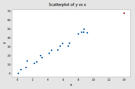
Example 11-4 Section
One last example! Do you think the following influence4 data set contains any outliers? Or, any high-leverage data points?
That's right — in this case, the red data point is most certainly an outlier and has high leverage! The red data point does not follow the general trend of the rest of the data and it also has an extreme x value. And, in this case, the red data point is influential. The two best-fitting lines — one obtained when the red data point is included and one obtained when the red data point is excluded:
are (not surprisingly) substantially different. The solid line represents the estimated regression equation with the red data point included, while the dashed line represents the estimated regression equation with the red data point taken excluded. The existence of the red data point significantly reduces the slope of the regression line — dropping it from 5.117 to 3.320.
Do the two samples yield different results when testing \(H_0 \colon \beta_1 = 0\)? Well, we obtain the following output when the red data point is included:
Model Summary
| S | R-sq | R-sq(adj) | R-sq(pred) |
|---|---|---|---|
| 10.4459 | 55.19% | 52.84% | 19.11% |
Model Summary
| Term | Coef | SE Coef | T-Value | P-Value | VIF |
|---|---|---|---|---|---|
| Constant | 8.50 | 4.22 | 2.01 | 0.058 | |
| x | 3.320 | 0.686 | 4.484 | 0.000 | 1.00 |
Regression Equation
\(\widehat{y} = 8.50 + 3.320 x\)
and the following output when the red data point is excluded:
Model Summary
| S | R-sq | R-sq(adj) | R-sq(pred) |
|---|---|---|---|
| 2.59199 | 97.32% | 97.17% | 96.63% |
Model Summary
| Term | Coef | SE Coef | T-Value | P-Value | VIF |
|---|---|---|---|---|---|
| Constant | 1.73 | 1.12 | 1.55 | 0.140 | |
| x | 5.117 | 0.200 | 25.55 | 0.000 | 1.00 |
Regression Equation
\(\widehat{y} = 1.73 + 5.117 x\)
What impact does the red data point have on our regression analysis here? In summary:
- The \(R^{2}\) value has decreased substantially from 97.32% to 55.19%. If we include the red data point, we conclude that the relationship between y and x is only moderately strong, whereas if we exclude the red data point, we conclude that the relationship between y and x is very strong.
- The standard error of \(b_1\) is almost 3.5 times larger when the red data point is included — increasing from 0.200 to 0.686. This increase would have a substantial effect on the width of our confidence interval for \(\beta_1\). Again, the increase is because the red data point is an outlier — in the y direction.
- In each case, the P-value for testing \(H_0 \colon \beta_1 = 0\) is less than 0.001. In both cases, we can conclude that there is sufficient evidence at the 0.05 level to conclude that, in the population, x is related to y. Note, however, that the t-statistic decreases dramatically from 25.55 to 4.84 upon inclusion of the red data point.
Here, the predicted responses and estimated slope coefficients are clearly affected by the presence of the red data point. While the data point did not affect the significance of the hypothesis test, the t-statistic did change dramatically. In this case, the red data point is deemed both high leverage and an outlier, and it turned out to be influential too.
Summary Section
The above examples — through the use of simple plots — have highlighted the distinction between outliers and high-leverage data points. There were outliers in examples 2 and 4. There were high-leverage data points in examples 3 and 4. However, only in example 4 did the data point that was both an outlier and a high leverage point turn out to be influential. That is, not every outlier or high-leverage data point strongly influences the regression analysis. It is your job as a regression analyst to always determine if your regression analysis is unduly influenced by one or more data points.
Of course, the easy situation occurs for simple linear regression, when we can rely on simple scatter plots to elucidate matters. Unfortunately, we don't have that luxury in the case of multiple linear regression. In that situation, we have to rely on various measures to help us determine whether a data point is an outlier, high leverage, or both. Once we've identified such points we then need to see if the points are actually influential. We'll learn how to do all this in the next few sections!