To complement the graphical methods just considered for assessing residual normality, we can perform a hypothesis test in which the null hypothesis is that the errors have a normal distribution. A large p-value and hence failure to reject this null hypothesis is a good result. It means that it is reasonable to assume that the errors have a normal distribution. Typically, assessment of the appropriate residual plots is sufficient to diagnose deviations from normality. However, a more rigorous and formal quantification of normality may be requested. So this section provides a discussion of some common testing procedures (of which there are many) for normality. For each test discussed below, the formal hypothesis test is written as:
\(\begin{align*} \nonumber H_{0}&\colon \textrm{the errors follow a normal distribution} \\ \nonumber H_{A}&\colon \textrm{the errors do not follow a normal distribution}. \end{align*}\)
While hypothesis tests are usually constructed to reject the null hypothesis, this is a case where we actually hope we fail to reject the null hypothesis as this would mean that the errors follow a normal distribution.
Anderson-Darling Test Section
The Anderson-Darling Test measures the area between a fitted line (based on the chosen distribution) and a nonparametric step function (based on the plot points). The statistic is a squared distance that is weighted more heavily in the tails of the distribution. Smaller Anderson-Darling values indicate that the distribution fits the data better. The test statistic is given by:
\(\begin{equation*} A^{2}=-n-\sum_{i=1}^{n}\frac{2i-1}{n}(\log \textrm{F}(e_{i})+\log (1-\textrm{F}(e_{n+1-i}))), \end{equation*}\)
where \(\textrm{F}(\cdot)\) is the cumulative distribution of the normal distribution. The test statistic is compared against the critical values from a normal distribution in order to determine the p-value.
The Anderson-Darling test is available in some statistical software. To illustrate here's statistical software output for the example on IQ and physical characteristics from Lesson 5 (IQ Size data), where we've fit a model with PIQ as the response and Brain and Height as the predictors:
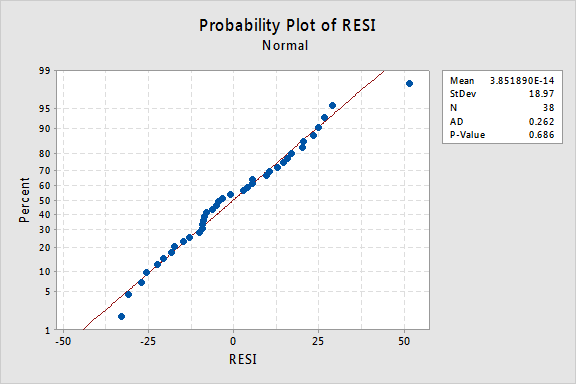
Since the Anderson-Darling test statistic is 0.262 with an associated p-value of 0.686, we fail to reject the null hypothesis and conclude that it is reasonable to assume that the errors have a normal distribution
Shapiro-Wilk Test Section
The Shapiro-Wilk Test uses the test statistic
\(\begin{equation*} W=\dfrac{\biggl(\sum_{i=1}^{n}a_{i}e_{(i)}\biggr)^{2}}{\sum_{i=1}^{n}(e_{i}-\bar{e})^{2}}, \end{equation*} \)
where \(e_{i}\) pertains to the \(i^{th}\) largest value of the error terms and the \(a_i\) values are calculated using the means, variances, and covariances of the \(e_{i}\). W is compared against tabulated values of this statistic's distribution. Small values of W will lead to the rejection of the null hypothesis.
The Shapiro-Wilk test is available in some statistical software. For the IQ and physical characteristics model with PIQ as the response and Brain and Height as the predictors, the value of the test statistic is 0.976 with an associated p-value of 0.576, which leads to the same conclusion as for the Anderson-Darling test.
Ryan-Joiner Test Section
The Ryan-Joiner Test is a simpler alternative to the Shapiro-Wilk test. The test statistic is actually a correlation coefficient calculated by
\(\begin{equation*} R_{p}=\dfrac{\sum_{i=1}^{n}e_{(i)}z_{(i)}}{\sqrt{s^{2}(n-1)\sum_{i=1}^{n}z_{(i)}^2}}, \end{equation*}\)
where the \(z_{(i)}\) values are the z-score values (i.e., normal values) of the corresponding \(e_{(i)}\) value and \(s^{2}\) is the sample variance. Values of \(R_{p}\) closer to 1 indicate that the errors are normally distributed.
The Ryan-Joiner test is available in some statistical software. For the IQ and physical characteristics model with PIQ as the response and Brain and Height as the predictors, the value of the test statistic is 0.988 with an associated p-value > 0.1, which leads to the same conclusion as for the Anderson-Darling test.
Kolmogorov-Smirnov Test Section
The Kolmogorov-Smirnov Test (also known as the Lilliefors Test) compares the empirical cumulative distribution function of sample data with the distribution expected if the data were normal. If this observed difference is sufficiently large, the test will reject the null hypothesis of population normality. The test statistic is given by:
\(\begin{equation*} D=\max(D^{+},D^{-}), \end{equation*}\)
where
\(\begin{align*} D^{+}&=\max_{i}(i/n-\textrm{F}(e_{(i)}))\\ D^{-}&=\max_{i}(\textrm{F}(e_{(i)})-(i-1)/n), \end{align*}\)
The test statistic is compared against the critical values from a normal distribution in order to determine the p-value.
The Kolmogorov-Smirnov test is available in some statistical software. For the IQ and physical characteristics model with PIQ as the response and Brain and Height as the predictors, the value of the test statistic is 0.097 with an associated p-value of 0.490, which leads to the same conclusion as for the Anderson-Darling test.