In order to get a handle on this multicollinearity thing, let's first investigate the effects that uncorrelated predictors have on regression analyses. To do so, we'll investigate a "contrived" data set, in which the predictors are perfectly uncorrelated. Then, we'll investigate the second example of a "real" data set, in which the predictors are nearly uncorrelated. Our two investigations will allow us to summarize the effects that uncorrelated predictors have on regression analyses.
Then, on the next page, we'll investigate the effects that highly correlated predictors have on regression analyses. In doing so, we'll learn — and therefore be able to summarize — the various effects multicollinearity has on regression analyses.
What is the effect on regression analyses if the predictors are perfectly uncorrelated?
Consider the following matrix plot of the response y and two predictors \(x_{1}\) and \(x_{2}\), of a contrived data set (Uncorrelated Predictors data set), in which the predictors are perfectly uncorrelated:
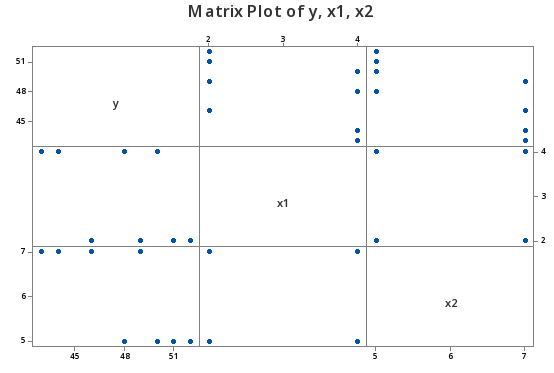
As you can see there is no apparent relationship at all between the predictors \(x_{1}\) and \(x_{2}\). That is, the correlation between \(x_{1}\) and \(x_{2}\) is zero:
Pearson correlation of x1 and x2 = 0.000
suggesting the two predictors are perfectly uncorrelated.
Now, let's just proceed quickly through the output of a series of regression analyses collecting various pieces of information along the way. When we're done, we'll review what we learned by collating the various items in a summary table.
The regression of the response y on the predictor \(x_{1}\):
Regression Analysis: y versus x1
Analysis of Variance
| Source | DF | Seq SS | Seq MS | F-Value | P-Value |
|---|---|---|---|---|---|
| Regression | 1 | 21.13 | 21.125 | 2.36 | 0.176 |
| x1 | 1 | 21.13 | 21.125 | 2.36 | 0.176 |
| Error | 6 | 53.75 | 8.958 | ||
| Total | 7 | 74.88 |
Model Summary
| S | R-sq | R-sq(adj) | R-sq(pred) |
|---|---|---|---|
| 2.99305 | 28.21% | 16.25% | 0.00% |
Coefficients
| Term | Coef | SE Coef | T-Value | P-Value | VIF |
|---|---|---|---|---|---|
| Constant | 52.75 | 3.35 | 15.76 | 0.000 | |
| x1 | -1.62 | 1.06 | -1.54 | 0.176 | 1.00 |
Regression Equation
\(\widehat{y} = 52.75 - 1.62 x1\)
yields the estimated coefficient \(b_{1}\) = -1.62, the standard error se(\(b_{1}\)) = 1.06, and the regression sum of squares SSR(\(x_{1}\)) = 21.13.
The regression of the response y on the predictor \(x_{2}\):
Regression Analysis: y versus x2
Analysis of Variance
| Source | DF | Seq SS | Seq MS | F-Value | P-Value |
|---|---|---|---|---|---|
| Regression | 1 | 45.13 | 45.125 | 9.10 | 0.023 |
| x2 | 1 | 45.13 | 45.125 | 9.10 | 0.023 |
| Error | 6 | 29.75 | 4.958 | ||
| Total | 7 | 74.88 |
Model Summary
| S | R-sq | R-sq(adj) | R-sq(pred) |
|---|---|---|---|
| 2.22673 | 60.27% | 53.64% | 29.36% |
Coefficients
| Term | Coef | SE Coef | T-Value | P-Value | VIF |
|---|---|---|---|---|---|
| Constant | 62.13 | 4.79 | 12.97 | 0.000 | |
| x2 | -2.375 | 0.787 | -3.02 | 0.023 | 1.00 |
Regression Equation
\(\widehat{y} = 62.13 - 2.375 x2\)
yields the estimated coefficient \(b_{2}\) = -2.375, the standard error se(\(b_{2}\)) = 0.787, and the regression sum of squares SSR(\(x_{2}\)) = 45.13.
The regression of the response y on the predictors \(x_{1 }\) and \(x_{2}\) (in that order):
Regression Analysis: y versus x1, x2
Analysis of Variance
| Source | DF | Seq SS | Seq MS | F-Value | P-Value |
|---|---|---|---|---|---|
| Regression | 2 | 66.250 | 33.125 | 19.20 | 0.005 |
| x1 | 1 | 21.125 | 21.125 | 12.25 | 0.017 |
| x2 | 1 | 45.125 | 45.125 | 26.16 | 0.004 |
| Error | 5 | 8.625 | 1.725 | ||
| Lack-of-Fit | 1 | 1.125 | 1.125 | 0.60 | 0.482 |
| Pure Error | 4 | 7.500 | 1.875 | ||
| Total | 7 | 74.875 |
Model Summary
| S | R-sq | R-sq(adj) | R-sq(pred) |
|---|---|---|---|
| 1.31339 | 88.48% | 83.87% | 70.51% |
Coefficients
| Term | Coef | SE Coef | T-Value | P-Value | VIF |
|---|---|---|---|---|---|
| Constant | 67.00 | 3.15 | 21.27 | 0.000 | |
| x1 | -1.625 | 0.464 | -3.50 | 0.017 | 1.00 |
| x2 | -2.375 | 0.464 | -5.11 | 0.004 | 1.00 |
Regression Equation
\(\widehat{y} = 67.00 - 1.625 x1 - 2.375 x2\)
yields the estimated coefficients \(b_{1}\) = -1.625 and \(b_{2}\) = -2.375, the standard errors se(\(b_{1}\)) = 0.464 and se(\(b_{2}\)) = 0.464, and the sequential sum of squares SSR(\(x_{2}\)|\(x_{1}\)) = 45.125.
The regression of the response y on the predictors \(x_{2 }\) and \(x_{1}\) (in that order):
Regression Analysis: y versus x2, x1
Analysis of Variance
| Source | DF | Seq SS | Seq MS | F-Value | P-Value |
|---|---|---|---|---|---|
| Regression | 2 | 66.250 | 33.125 | 19.20 | 0.005 |
| x2 | 1 | 45.125 | 45.125 | 26.16 | 0.004 |
| x1 | 1 | 21.125 | 21.125 | 12.25 | 0.017 |
| Error | 5 | 8.625 | 1.725 | ||
| Lack-of-Fit | 1 | 1.125 | 1.125 | 0.60 | 0.482 |
| Pure Error | 4 | 7.500 | 1.875 | ||
| Total | 7 | 74.875 |
Model Summary
| S | R-sq | R-sq(adj) | R-sq(pred) |
|---|---|---|---|
| 1.31339 | 88.48% | 83.87% | 70.51% |
Coefficients
| Term | Coef | SE Coef | T-Value | P-Value | VIF |
|---|---|---|---|---|---|
| Constant | 67.00 | 3.15 | 21.27 | 0.000 | |
| x2 | -2.375 | 0.464 | -5.11 | 0.004 | 1.00 |
| x1 | -1.625 | 0.464 | -3.50 | 0.017 | 1.00 |
Regression Equation
\(\widehat{y} = 67.00 - 2.375 x2 - 1.625 x1\)
yields the estimated coefficients \(b_{1}\) = -1.625 and \(b_{2}\) = -2.375, the standard errors se(\(b_{1}\)) = 0.464 and se(\(b_{2}\)) = 0.464, and the sequential sum of squares SSR(\(x_{1}\)|\(x_{2}\)) = 21.125.
Okay — as promised — compiling the results in a summary table, we obtain:
|
Model |
\(b_{1}\) | se(\(b_{1}\)) | \(b_{2}\) | se(\(b_{2}\)) | Seq SS |
|---|---|---|---|---|---|
| \(x_{1}\) only | -1.62 | 1.06 | --- | --- | SSR(\(x_{1}\)) 21.13 |
| \(x_{2}\) only | --- | --- | -2.375 | 45.13 | SSR(\(x_{2}\)) 45.13 |
| \(x_{1}\), \(x_{2}\) (in order) |
-1.625 | 0.464 | -2.375 | 0.464 | SSR(\(x_{2}\)|\(x_{1}\)) 21.125 |
| \(x_{2}\), \(x_{1}\) (in order) |
-1.625 | 0.464 | -2.375 | 0.464 | SSR(\(x_{1}\)|\(x_{2}\)) 45.125 |
What do we observe?
- The estimated slope coefficients \(b_{1}\) and \(b_{2}\) are the same regardless of the model used.
- The standard errors se(\(b_{1}\)) and se(\(b_{2}\)) don't change much at all from model to model.
- The sum of squares SSR(\(x_{1}\)) is the same as the sequential sum of squares SSR(\(x_{1}\)|\(x_{2}\)). The sum of squares SSR(\(x_{2}\)) is the same as the sequential sum of squares SSR(\(x_{2}\)|\(x_{1}\)).
These all seem to be good things! Because the slope estimates stay the same, the effect on the response ascribed to a predictor doesn't depend on the other predictors in the model. Because SSR(\(x_{1}\)) = SSR(\(x_{1}\)|\(x_{2}\)), the marginal contribution that \(x_{1}\) has in reducing the variability in the response y doesn't depend on the predictor \(x_{2}\). Similarly, because SSR(\(x_{2}\)) = SSR(\(x_{2}\)|\(x_{1}\)), the marginal contribution that \(x_{2}\) has in reducing the variability in the response y doesn't depend on the predictor \(x_{1}\).
These are the things we can hope for in regression analysis — but, then reality sets in! Recall that we obtained the above results for a contrived data set, in which the predictors are perfectly uncorrelated. Do we get similar results for real data with only nearly uncorrelated predictors? Let's see!
What is the effect on regression analyses if the predictors are nearly uncorrelated? Section
To investigate this question, let's go back and take a look at the blood pressure data set (Blood Pressure data set). In particular, let's focus on the relationships among the response y = BP and the predictors \(x_{3}\) = BSA and \(x_{6}\) = Stress:
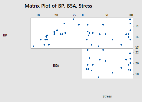
As the above matrix plot and the following correlation matrix suggest:
Correlation: BP, Age, Weight, BSA, Dur, Pulse, Stress
| BP | Age | Weight | BSA | Dur | Pulse | |
|---|---|---|---|---|---|---|
| Age | 0.659 | |||||
| Weight | 0.950 | 0.407 | ||||
| BSA | 0.866 | 0.378 | 0.875 | |||
| Dur | 0.293 | 0.344 | 0.201 | 0.131 | ||
| Pulse | 0.721 | 0.619 | 0.659 | 0.465 | 0.402 | |
| Stress | 0.164 | 0.368 | 0.034 | 0.018 | 0.312 | 0.506 |
there appears to be a strong relationship between y = BP and the predictor \(x_{3}\) = BSA (r = 0.866), a weak relationship between y = BP and \(x_{6}\) = Stress (r = 0.164), and an almost non-existent relationship between \(x_{3}\) = BSA and \(x_{6}\) = Stress (r = 0.018). That is, the two predictors are nearly perfectly uncorrelated.
What effect do these nearly perfectly uncorrelated predictors have on regression analyses? Let's proceed similarly through the output of a series of regression analyses collecting various pieces of information along the way. When we're done, we'll review what we learned by collating the various items in a summary table.
The regression of the response y = BP on the predictor \(x_{6}\)= Stress:
Analysis of Variance
| Source | DF | Seq SS | Seq MS | F-Value | P-Value |
|---|---|---|---|---|---|
| Regression | 1 | 15.04 | 15.04 | 0.50 | 0.490 |
| Stress | 1 | 15.04 | 15.04 | 0.50 | 0.490 |
| Error | 18 | 544.96 | 30.28 | ||
| Lack-of-Fit | 14 | 457.79 | 32.70 | 1.50 | 0.374 |
| Pure Error | 4 | 87.17 | 21.79 | ||
| Total | 19 | 560.00 |
Coefficients
| Term | Coef | SE Coef | T-Value | P-Value | VIF |
|---|---|---|---|---|---|
| Constant | 112.72 | 2.19 | 51.39 | 0.000 | |
| Stress | 0.0240 | 0.0340 | 0.70 | 0.490 | 1.00 |
Regression Equation
\(\widehat{BP} = 112.72 + 0.0240 Stress\)
yields the estimated coefficient \(b_{6}\) = 0.0240, the standard error se(\(b_{6}\)) = 0.0340, and the regression sum of squares SSR(\(x_{6}\)) = 15.04.
The regression of the response y = BP on the predictor \(x_{3 }\)= BSA:
Analysis of Variance
| Source | DF | Seq SS | Seq MS | F-Value | P-Value |
|---|---|---|---|---|---|
| Regression | 1 | 419.858 | 419.858 | 53.93 | 0.000 |
| BSA | 1 | 419.858 | 419.858 | 53.93 | 0.000 |
| Error | 18 | 140.142 | 7.786 | ||
| Lack-of-Fit | 13 | 133.642 | 10.280 | 7.91 | 0.016 |
| Pure Error | 5 | 6.500 | 1.300 | ||
| Total | 19 | 560.000 |
Coefficients
| Term | Coef | SE Coef | T-Value | P-Value | VIF |
|---|---|---|---|---|---|
| Constant | 49.50 | 4.65 | 10.63 | 0.000 | |
| BSA | 34.44 | 4.69 | 7.34 | 0.000 | 1.00 |
Regression Equation
\(\widehat{BP} = 45.18 + 34.44 BSA\)
yields the estimated coefficient \(b_{3}\) = 34.44, the standard error se(\(b_{3}\)) = 4.69, and the regression sum of squares SSR(\(x_{3}\)) = 419.858.
The regression of the response y = BP on the predictors \(x_{6}\)= Stress and \(x_{3}\)= BSA (in that order):
Analysis of Variance
| Source | DF | Seq SS | Seq MS | F-Value | P-Value |
|---|---|---|---|---|---|
| Regression | 2 | 432.12 | 216.058 | 28.72 | 0.000 |
| Stress | 1 | 15.04 | 15.044 | 2.00 | 0.175 |
| BSA | 1 | 417.07 | 417.073 | 55.44 | 0.000 |
| Error | 17 | 127.88 | 7.523 | ||
| Total | 19 | 560.00 |
Coefficients
| Term | Coef | SE Coef | T-Value | P-Value | VIF |
|---|---|---|---|---|---|
| Constant | 44.24 | 9.26 | 4.78 | 0.000 | |
| Stress | 0.0217 | 0.0170 | 1.28 | 0.219 | 1.00 |
| BSA | 34.33 | 4.61 | 7.45 | 0.000 | 1.00 |
Regression Equation
\(\widehat{y} = 44.24 + 0.0217 Stress + 34.33 BSA\)
yields the estimated coefficients \(b_{6}\) = 0.0217 and \(b_{3}\) = 34.33, the standard errors se(\(b_{6}\)) = 0.0170 and se(\(b_{2}\)) = 4.61, and the sequential sum of squares SSR(\(x_{3}\)|\(x_{6}\)) = 417.07.
Finally, the regression of the response y = BP on the predictors \(x_{3 }\)= BSA and \(x_{6}\)= Stress (in that order):
Analysis of Variance
| Source | DF | Seq SS | Seq MS | F-Value | P-Value |
|---|---|---|---|---|---|
| Regression | 2 | 432.12 | 216.058 | 28.72 | 0.000 |
| BSA | 1 | 419.86 | 419.858 | 55.81 | 0.000 |
| Stress | 1 | 12.26 | 12.259 | 1.63 | 0.219 |
| Error | 6 | 104.000 | 17.333 | ||
| Total | 7 | 112.000 |
Coefficients
| Term | Coef | SE Coef | T-Value | P-Value | VIF |
|---|---|---|---|---|---|
| Constant | 44.24 | 9.26 | 4.78 | 0.000 | |
| BSA | 34.33 | 4.61 | 7.45 | 0.000 | 1.00 |
| Stress | 0.0217 | 0.0170 | 1.28 | 0.219 | 1.00 |
Regression Equation
\(\widehat{BP} = 44.24 + 34.33 BSA + 0.0217 Stress\)
yields the estimated coefficients \(b_{6}\) = 0.0217 and \(b_{3}\) = 34.33, the standard errors se(\(b_{6}\)) = 0.0170 and se(\(b_{2}\)) = 4.61, and the sequential sum of squares SSR(\(x_{6}\)|\(x_{3}\)) = 12.26.
Again — as promised — compiling the results in a summary table, we obtain:
| Model | \(b_{6}\) | se(\(b_{6}\)) | \(b_{3}\) | se(\(b_{3}\)) | Seq SS |
|---|---|---|---|---|---|
| \(x_{6}\) only | 0.0240 | 0.0340 | --- | --- | SSR(\(x_{6}\)) 15.04 |
| \(x_{3}\) only | --- | --- | 34.44 | 4.69 | SSR(\(x_{3}\)) 419.858 |
| \(x_{6}\), \(x_{3}\) (in order) |
0.0217 | 0.0170 | 34.33 | 4.61 | SSR(\(x_{3}\)|\(x_{6}\)) 417.07 |
| \(x_{3}\), \(x_{6}\) (in order) |
0.0217 | 0.0170 | 34.33 | 4.61 | SSR(\(x_{6}\)|\(x_{3}\)) 12.26 |
What do we observe? If the predictors are nearly perfectly uncorrelated:
- We don't get identical, but very similar slope estimates \(b_{3}\) and \(b_{6}\), regardless of the predictors in the model.
- The sum of squares SSR(\(x_{3}\)) is not the same, but very similar to the sequential sum of squares SSR(\(x_{3}\)|\(x_{6}\)).
- The sum of squares SSR(\(x_{6}\)) is not the same, but very similar to the sequential sum of squares SSR(\(x_{6}\)|\(x_{3}\)).
Again, these are all good things! In short, the effect on the response ascribed to a predictor is similar regardless of the other predictors in the model. And, the marginal contribution of a predictor doesn't appear to depend much on the other predictors in the model.
Try it!
Uncorrelated predictors Section
Effect of perfectly uncorrelated predictor variables.
This exercise reviews the benefits of having perfectly uncorrelated predictor variables. The results of this exercise demonstrate a strong argument for conducting "designed experiments" in which the researcher sets the levels of the predictor variables in advance, as opposed to conducting an "observational study" in which the researcher merely observes the levels of the predictor variables as they happen. Unfortunately, many regression analyses are conducted on observational data rather than experimental data, limiting the strength of the conclusions that can be drawn from the data. As this exercise demonstrates, you should conduct an experiment, whenever possible, not an observational study. Use the (contrived) data stored in the Uncorrelated Predictor data set to complete this lab exercise.
-
Using the Stat >> Basic Statistics >> Correlation... command in Minitab, calculate the correlation coefficient between \(X_{1}\) and \(X_{2}\). Are the two variables perfectly uncorrelated?Correlation = 0 so, yes, the two variables are perfectly uncorrelated
-
Fit the simple linear regression model with y as the response and \(x_{1}\) as the single predictor:
- What is the value of the estimated slope coefficient \(b_{1}\)?
- What is the regression sum of squares, SSR (\(X_{1}\)), when \(x_{1}\) is the only predictor in the model?
Estimated slope coefficient \(b_1 = -5.80\)
\(SSR(X_1) = 336.40\)
-
Now, fit the simple linear regression model with y as the response and \(x_{2}\) as the single predictor:
- What is the value of the estimated slope coefficient \(b_{2}\)?
- What is the regression sum of squares, SSR (\(X_{2}\)), when \(x_{2}\) is the only predictor in the model?
Estimated slope coefficient \(b_2 = 1.36\).
\(SSR(X_2) = 206.2\).
-
Now, fit the multiple linear regression model with y as the response and \(x_{1}\) as the first predictor and \(x_{2}\) as the second predictor:
- What is the value of the estimated slope coefficient \(b_{1}\)? Is the estimate \(b_{1}\) different than that obtained when \(x_{1}\) was the only predictor in the model?
- What is the value of the estimated slope coefficient \(b_{2}\)? Is the estimate \(b_{2}\) different than that obtained when \(x_{2}\) was the only predictor in the model?
- What is the sequential sum of squares, SSR (\(X_{2}\)|\(X_{1}\))? Does the reduction in the error sum of squares when x2}\) is added to the model depend on whether \(x_{1}\) is already in the model?
Estimated slope coefficient \(b_1 = -5.80\), the same as before.
Estimated slope coefficient \(b_2 = 1.36\), the same as before.
\(SSR(X_2|X_1) = 206.2 = SSR(X_2)\), so this doesn’t depend on whether \(X_1\) is already in the model.
-
Now, fit the multiple linear regression model with y as the response and \(x_{2}\) as the first predictor, and \(x_{1}\) as the second predictor:
- What is the sequential sum of squares, SSR (\(X_{1}\)|\(X_{2}\))? Does the reduction in the error sum of squares when \(x_{1}\) is added to the model depend on whether \(x_{2}\) is already in the model?
\(SSR(X_2|X_1) = 336.4 = SSR(X_1)\), so this doesn’t depend on whether \(X_2\) is already in the model.
-
When the predictor variables are perfectly uncorrelated, is it possible to quantify the effect a predictor has on the response without regard to the other predictors?
Yes -
In what way does this exercise demonstrate the benefits of conducting a designed experiment rather than an observational study?
It is possible to quantify the effect a predictor has on the response regardless of whether other (uncorrelated) predictors have been included