Example 14-3: Employee Data Section

The next data set gives the number of employees (in thousands) for a metal fabricator and one of their primary vendors for each month over a 5-year period, so n = 60 (Employee data). A simple linear regression analysis was implemented:
\(\begin{equation*} y_{t}=\beta_{0}+\beta_{1}x_{t}+\epsilon_{t}, \end{equation*}\)
where \(y_{t}\) and \(x_{t}\) are the number of employees during time period t at the metal fabricator and vendor, respectively.
A plot of the number of employees at the fabricator versus the number of employees at the vendor with the ordinary least squares regression line overlaid is given below in plot (a). A scatterplot of the residuals versus t (the time ordering) is given in plot (b).
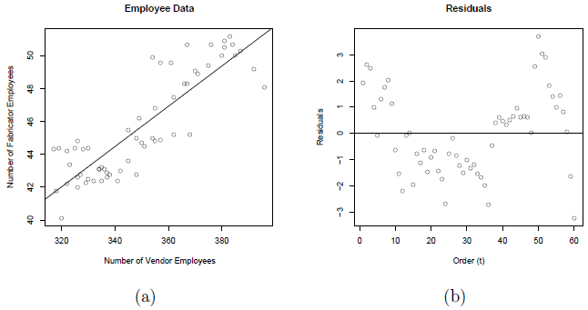
Notice the non-random trend suggestive of autocorrelated errors in the scatterplot. The estimated equation is \(y_{t}=2.85+0.12244x_{t}\), which is given in the following summary output:
Model Summary
| S | R-sq | R-sq(adj) | R-sq(pred) |
|---|---|---|---|
| 1.58979 | 74.43% | 73.99% | 72.54% |
Coefficients
| Term | Coef | SE Coef | T-Value | P-Value | VIF |
|---|---|---|---|---|---|
| Constant | 2.85 | 3.30 | 0.86 | 0.392 | |
| vendor | 0.12244 | 0.00942 | 12.99 | 0.000 | 1.00 |
Regression Equation
metal = 2.85 + 0.12244 vendor
The plot below gives the PACF plot of the residuals, which helps us decide the lag values. (Minitab: Store the residuals from the regression model fit then select Stat > Time Series > Partial Autocorrelation and use the stored residuals as the "Series.")
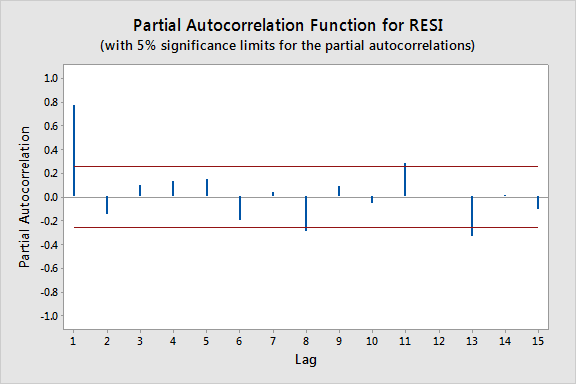
In particular, it looks like there is a lag of 1 since the lag-1 partial autocorrelation is so large and way beyond the "5% significance limits" shown by the red lines. (The partial autocorrelations at lags 8, 11, and 13 are only slightly beyond the limits and would lead to an overly complex model at this stage of the analysis.) We can also obtain the output from the Durbin-Watson test for serial correlation (Minitab: click the "Results" button in the Regression Dialog and check "Durbin-Watson statistic."):
Durbin-Watson Statistic
Durbin-Watson Statistic = 0.359240
To find the p-value for this test statistic we need to look up a Durbin-Watson critical values table, which in this case indicates a highly significant p-value of approximately 0. (In general Durbin-Watson statistics close to 0 suggest significant positive autocorrelation.) A lag of 1 appears appropriate.
Since we decide upon using AR(1) errors, we will have to use one of the procedures we discussed earlier. In particular, we will use the Cochrane-Orcutt procedure. Start by fitting a simple linear regression model with a response variable equal to the residuals from the model above and a predictor variable equal to the lag-1 residuals and no intercept to obtain the slope estimate, r = 0.831385.
Now, transform to \(y_{t}^{*}=y_{t}-ry_{t-1}\) and \(x_{t}^{*}=x_{t}-rx_{t-1}\). Perform a simple linear regression of \(y_{t}^{*}\) on \(x_{t}^{*}\). The resulting regression estimates from the Cochrane-Orcutt procedure are:
\(\begin{align*} \hat{\beta}_{1}^{*}&=0.0479=\hat{\beta}_{1} \\ \hat{\beta}_{0}^{*}&=4.876\Rightarrow\hat{\beta}_{0}=\frac{4.876}{1-0.831385}=28.918. \end{align*}\)
The corresponding standard errors are:
\(\begin{align*} \mbox{s.e.}(\hat{\beta}_{1}^{*})&=0.0130=\mbox{s.e.}(\hat{\beta}_{1})\\ \mbox{s.e.}(\hat{\beta}_{0}^{*})&=0.787\Rightarrow\mbox{s.e.}(\hat{\beta}_{0})=\frac{0.787}{1-0.831385}=4.667. \end{align*}\)
Notice that the correct standard errors (from the Cochrane-Orcutt procedure) are larger than the incorrect values from the simple linear regression on the original data. If ordinary least squares estimation is used when the errors are autocorrelated, the standard errors often are underestimated. It is also important to note that this does not always happen. Underestimation of the standard errors is an "on average" tendency overall problem.
Example 14-4: Oil Data Section
The data are from U.S. oil and gas price index values for 82 months (dataset no longer available). There is a strong linear pattern for the relationship between the two variables, as can be seen below.
We start the analysis by doing a simple linear regression. Minitab results for this analysis are given below.
Coefficients
| Predictor | Coef | SE Coef | T-Value | P-Value |
|---|---|---|---|---|
| Constant | -31.349 | 5.219 | -6.01 | 0.000 |
| Oil | 1.17677 | 0.02305 | 51.05 | 0.000 |
Regression Equation
Gas = -31.3 + 1.18 Oil
The residuals in time order show a dependent pattern (see the plot below).
The slow cyclical pattern that we see happens because there is a tendency for residuals to keep the same algebraic sign for several consecutive months. We also used Stat >> Time Series >> Lag to create a column of the lag 1 residuals. The correlation coefficient between the residuals and the lagged residuals is calculated to be 0.829 (and is calculated using Stat >> Basic Stats >> Correlation, which can be seen at the bottom of the figure above).
So, the overall analysis strategy in presence of autocorrelated errors is as follows:
- Do an ordinary regression. Identify the difficulty in the model (autocorrelated errors).
- Using the stored residuals from the linear regression, use regression to estimate the model for the errors, \(\epsilon_t = \rho\epsilon_{t-1} + u_t\) where the \(u_t\) are iid with mean 0 and variance \(\sigma^{2}\).
- Adjust the parameter estimates and their standard errors from the original regression.
A Method for Adjusting the Original Parameter Estimates (Cochrane-Orcutt Method)
- Let \(\hat{\rho}\) = estimated lag 1 autocorrelation in the residuals from the ordinary regression (in the U.S. oil example, \(\hat{\rho} = 0.829\)).
- Let \({y^{*}}_t = y_t − \hat{\rho} y_{t-1}\). This will be used as a response variable.
- Let \({x^{*}}_t = x_t − \hat{\rho} x_{t-1}\). This will be used as a predictor variable.
- Do an “ordinary” regression between \({y^*}_t\) and \({x^*}_t\) . This model should have time-independent residuals.
- The sample slope from the regression directly estimates \(\beta_1\), the slope of the relationship between the original y and x.
- The correct estimate of the intercept for the original model y versus x relationship is calculated as \(\beta_0=\hat{\beta}_0^* / (1-\hat{\rho})\), where \(\hat{\beta}_0\) is the sample intercept obtained from the regression done with the modified variables.
Returning to the U.S. oil data, the value of \(\hat{\rho} = 0.829\) and the modified variables are \(\mathbf{ynew} = y_t − 0.829 y_{t-1}\) and \(\mathbf{xnew} = x_t −0.829 x_{t-1}\). The regression results are given below.
Coefficients
| Predictor | Coef | SE Coef | T | P |
|---|---|---|---|---|
| Constant | -1.412 | 2.529 | -0.56 | 0.578 |
| xnew | 1.08073 | 0.05960 | 18.13 | 0.000 |
Parameter Estimates for the Original Model
Our real goal is to estimate the original model \(y_t = \beta_0 +\beta_1 x_t + \epsilon_t\) . The estimates come from the results just given.
\(\hat{\beta}_1=1.08073\)
\(\hat{\beta}_0=\dfrac{-1.412}{1-0.829}=-8.2573\)
These estimates give the sample regression model:
\(y_t = −8.257 + 1.08073 x_t + \epsilon_t\)
with \(\epsilon_t = 0.829 \epsilon_{t-1} + u_t\) , where \(u_t\)’s are iid with mean 0 and variance \(\sigma^{2}\).
Correct Standard Errors for the Coefficients
- The correct standard error for the slope is taken directly from the regression with the modified variables.
- The correct standard error for the intercept is \(\text{s.e.}\hat{\beta}_0=\dfrac{\text{s.e.}\hat{\beta}_0^*}{1-\hat{\rho}}\).
Correct and incorrect estimates for the coefficients:
| Coefficient | Correct Estimate | Correct Standard Error |
|---|---|---|
| Intercept | −1.412 / (1−0.829) = −8.2573 | 2.529 / (1−0.829) = 14.79 |
| Slope | 1.08073 | 0.05960 |
| Incorrect Estimate | Incorrect Standard Error | |
| Intercept | -31.349 | 5.219 |
| Slope | 1.17677 | 0.02305 |
This table compares the correct standard errors to the incorrect estimates based on the ordinary regression. The “correct” estimates come from the work done in this section of the notes. The incorrect estimates are from the original regression estimates reported above. Notice that the correct standard errors are larger than the incorrect values here. If ordinary least squares estimation is used when the errors are autocorrelated, the standard errors often are underestimated. It is also important to note that this does not always happen. Overestimation of the standard errors is an “on average” tendency overall problem.
Forecasting Issues
When calculating forecasts for time series, it is important to utilize \(\epsilon_t = \rho \epsilon_{t-1} + u_t\) as part of the process. In the U.S. oil example,
\(F_t=\hat{y}_t + e_t = −8.257 + 1.08073 x_t + e_t = −8.257 + 1.08073 x_t + 0.829 e_{t-1}\)
Values of \(F_t\) are computed iteratively:
- Compute \(\hat{y}_1= −8.257 + 1.08073x_1\) and \(e_1=y_1-\hat{y}_1\).
- Compute \(\hat{y}_2= −8.257 + 1.08073x_2\) and use the value of \(e_1\) when computing \(F_2 = \hat{y}_2 + 0.829e_1\).
- Determine \(e_2=y_2-\hat{y}_2\).
- Compute \(\hat{y}_3= −8.257 + 1.08073x_3\) and use the value of \(e_2\) when computing \(F_3 = \hat{y}_3 + 0.829e_2\).
- Iterate.