Example 8-5: Piecewise linear regression model Section

We discuss what is called "piecewise linear regression models" here because they utilize interaction terms containing dummy variables.
Let's start with an example that demonstrates the need for using a piecewise approach to our linear regression model. Consider the following plot of the compressive strength (y) of n = 18 batches of concrete against the proportion of water (x) mixed in with the cement:
The estimated regression line —the solid line —appears to fit the data fairly well in some overall sense, but it is clear that we could do better. The residuals versus fits plot:
provides yet more evidence that our model needs work.
We could instead split our original scatter plot into two pieces —where the water-cement ratio is 70% —and fit two separate, but connected lines, one for each piece. As you can see, the estimated two-piece function, connected at 70% —the dashed line —appears to do a much better job of describing the trend in the data.
So, let's formulate a piecewise linear regression model for these data, in which there are two pieces connected at x = 70:
\(y_i=\beta_0+\beta_1x_{i1}+\beta_2(x_{i1}-70)x_{i2}+\epsilon_i\)
Alternatively, we could write our formulated piecewise model as:
\(y_i=\beta_0+\beta_1x_{i1}+\beta_2x_{i2}^{*}+\epsilon_i\)
where:
- \(y_i\) is the comprehensive strength, in pounds per square inch, of concrete batch i
- \(x_{i1}\) is the water-cement ratio, in %, of concrete batch i
- \(x_{i2}\) is a dummy variable \(\left( 0 , \text{ if } x_{i1} ≤ 70 \text{ and } 1 , \text{ if } x_{i1} > 70 \right)\) of concrete batch i
- \(x_{i2}*\) denotes the \(\left(x_{i1} - 70\right) x_{i2}\) the interaction term
and the independent error terms \(\epsilon_i\) follow a normal distribution with mean 0 and equal variance \(\sigma^{2}\).
With a little bit of algebra —
—we can see how the piecewise regression model as formulated above yields two separate linear functions connected at x = 70. Incidentally, the x-value at which the two pieces of the model connect is called the "knot value." For our example here, the knot value is 70.
Now, estimating our piecewise function in Minitab, we obtain:
The regression equation
strength = 7.79 - 0.0663 ratio - 0.101 x2*
| Predictor | Coef | SE Coef | T | P |
|---|---|---|---|---|
| Constant | 7.7920 | 0.6770 | 11.51 | 0.000 |
| ratio | -0.06633 | 0.01123 | -5.90 | 0.000 |
| x2* | -0.10119 | 0.02812 | -3.60 | 0.003 |
| Model Summary | ||
|---|---|---|
| S = 0.3286 | R-Sq = 93.8% | R-Sq(adj) = 93.0% |
Analysis of Variance
| Source | DF | SS | MS | F | P |
|---|---|---|---|---|---|
| Regression | 2 | 24.718 | 12.359 | 114.44 | 0.000 |
| Residual Error | 15 | 1.620 | 0.108 | ||
| Total | 17 | 26.338 |
With a little bit of algebra, we see how the estimated regression equation that Minitab reports:
Regression Equation
strength = 7.79 - 0.0663 ratio - 0.101 x2*yields two estimated regression lines, connected at x = 70, that fit the data quite well:
And, the residuals versus fits plot illustrates a significant improvement in the fit of the model:
Try It!
Piecewise linear regression Section
Shipment data. This exercise is intended to review the concept of piecewise linear regression. The basic idea behind piecewise linear regression is that if the data follow different linear trends over different regions of the data then we should model the regression function in "pieces." The pieces can be connected or not connected. Here, we'll fit a model in which the pieces are connected.
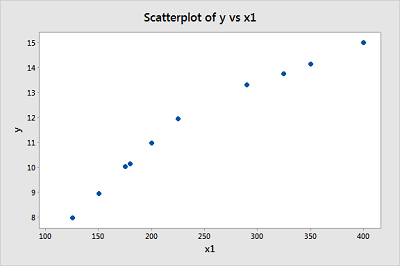
We'll use the Shipment dataset. An electronics company periodically imports shipments of a certain large part used as a component in several of its products. The size of the shipment varies depending on production schedules. For handling and distribution to assembly plants, shipments of size 250 thousand parts or less are sent to warehouse A; larger shipments are sent to warehouse B since this warehouse has specialized equipment that provides greater economies of scale for large shipments.
The data set contains information on the cost (y) of handling the shipment in the warehouse (in thousand dollars) and the size \(\left(x_1 \right)\) of the shipment (in thousand parts).
-
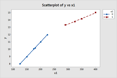
Create a scatter plot of the data with cost on the y-axis and size on the x-axis. (See Minitab Help: Creating a basic scatter plot). Based on the plot, does it seem reasonable that there are two different (but connected) regression functions — one when \(x_1 < 250\) and one when \(x_1 > 250\)?
-
Not surprisingly, we'll use a dummy variable and an interaction term to help define the piecewise linear regression model. Specifically, the model we'll fit is:
\(y_i = \beta_0 + \beta_1 x_{i1} + \beta_2 \left(x_{i1} - 250\right) x_{i2} + \epsilon_i\)
where \(x_{i1}\) is the size of the shipment and \(x_{i2} = 0\) if \(x_{i1} < 250\) and \(x_{i2} = 1\) if \(x_{i1} > 250\). We could also write this model as:
\(y_i = \beta0 + \beta_1 x_{i1} + \beta_2 {x^{*}}_{i2} + \epsilon_i\)
where \(x^*_{i2} = \left(x_{i1} - 250 \right) x_{i2}\). If we assume the data follow this model, what is the mean response function for shipments whose size is smaller than 250? And, what is the mean response function for shipments whose size is greater than 250? Do the two mean response functions have different slopes and connect when \(x_{i1} = 250\)?
\(\mu_Y = \beta_0 + \beta_1 x_1 + \beta_2 (x_1 - 250) x_2\)
\(\mu_Y|(x_1<250) = \beta_0 + \beta_1 x_1 + \beta_2 (x_1 - 250) (0) = \beta_0 + \beta_1 x_1\)
\(\mu_Y|(x_1>250) = \beta_0 + \beta_1 x_1 + \beta_2 (x_1 - 250) (1) = (\beta_0 - 250 \beta_2) + (\beta_1+\beta_2)x_1\)
When \(x_1=250, \beta_0 + \beta_1 x_1 = \beta_0 + 250\beta_1\)
When \(x_1=250, (\beta_0 - 250 \beta_2) + (\beta_1+\beta_2)(250) = \beta_0 + 250 \beta_1\)
-
You first need to set up the data set so that you can easily fit the model. In the data set, y denotes cost and \(x_1\) denotes the size. This is the easiest way to create the new variable, \(x*_{i2} = x_{1} ^{shift} x_2\), say:
- Use Minitab's calculator to create a new variable, \(x_1 ^{shift}\) , say, which equals \(x_1 - 250\).
- Use Minitab's Manip >> Code command (v16) or Data >> Recode >> To Numeric command (v17) to create \(x_2\). To do so, tell Minitab that you want to recode values in column x_{1} using the method "Recode range of values." Indicate that you want values from 0 to 250 to take on value 0 and values from 250 to 500 to take on value 1. Store the re-coded column in a specied column of the current worksheet named x2.
- Use Minitab's calculator to multiply \(x_1 ^{shift}\) by \(x_2\) to get \({x_1}^{shift} x_2\). Review the values obtained to convince yourself that they take on the values as defined. Then, fit the linear regression model with y as the response and \(x_1\) and \({x_1}^{shift} x_2\) as the predictors. What is the estimated regression function for shipments whose size < 250? for shipments whose size > 250?
\(\hat{y} = 3.214 + 0.038460 x_1 - 0.02477 x_1 \text{shift} x_2\)
\(\hat{y}|(x_1<250) = 3.214 + 0.038460 x_1 - 0.02477 (0) = 3.214 + 0.03846 x_1\)
\(\hat{y}|(x_1>250) = 3.214 + 0.038460 x_1 - 0.02477 (x_1-250) = (3.214 - 250(-0.02477)) + (0.038460-0.02477) x_1 = 9.4065 + 0.01369 x_1\)
-
Based on your estimated regression function, what is the predicted cost for a shipment with a size of 125? a size of 250? with a size of 400? Convince yourself that you get the same prediction for size = 250 regardless of which estimated regression function you use.
\(\hat{y}|(x_1=125) = 3.214 + 0.03846 (125) = 8.0215\)
\(\hat{y}|(x_1=250) = 3.214 + 0.03846 (250) = 12.8290\)
\(\hat{y}|(x_1=250) = 9.4065 + 0.01369 (250) = 12.8290\)
\(\hat{y}|(x_1=400) = 9.4065 + 0.01369 (400) = 14.8825\)
-
Using your predicted values for size = 125, 250, and 400, create another scatter plot of the data, but this time "annotate" the graph with the two connected lines. (Note that the F3 key should completely erase any previous work, such as annotation lines, in the Graph >> Plot command.) Do you think the piecewise linear regression model reasonably summarizes these data?