Let's start our investigation of the coefficient of determination, \(R^{2}\), by looking at two different examples — one example in which the relationship between the response y and the predictor x is very weak and a second example in which the relationship between the response y and the predictor x is fairly strong. If our measure is going to work well, it should be able to distinguish between these two very different situations.
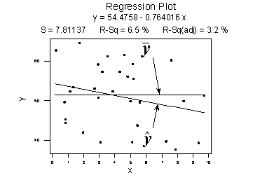
Here's a plot illustrating a very weak relationship between y and x. There are two lines on the plot, a horizontal line placed at the average response, \(\bar{y}\), and a shallow-sloped estimated regression line, \(\hat{y}\). Note that the slope of the estimated regression line is not very steep, suggesting that as the predictor x increases, there is not much of a change in the average response y. Also, note that the data points do not "hug" the estimated regression line:

\(SSR=\sum_{i=1}^{n}(\hat{y}_i -\bar{y})^2=119.1\)
\(SSE=\sum_{i=1}^{n}(y_i-\hat{y}_i)^2=1708.5\)
\(SSTO=\sum_{i=1}^{n}(y_i-\bar{y})^2=1827.6\)
The calculations on the right of the plot show contrasting "sums of squares" values:
- SSR is the "regression sum of squares" and quantifies how far the estimated sloped regression line, \(\hat{y}_i\), is from the horizontal "no relationship line," the sample mean or \(\bar{y}\).
- SSE is the "error sum of squares" and quantifies how much the data points, \(y_i\), vary around the estimated regression line, \(\hat{y}_i\).
- SSTO is the "total sum of squares" and quantifies how much the data points, \(y_i\), vary around their mean, \(\bar{y}\).
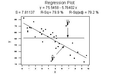
Contrast the above example with the following one in which the plot illustrates a fairly convincing relationship between y and x. The slope of the estimated regression line is much steeper, suggesting that as the predictor x increases, there is a fairly substantial change (decrease) in the response y. And, here, the data points do "hug" the estimated regression line:

\(SSR=\sum_{i=1}^{n}(\hat{y}_i-\bar{y})^2=6679.3\)
\(SSE=\sum_{i=1}^{n}(y_i-\hat{y}_i)^2=1708.5\)
\(SSTO=\sum_{i=1}^{n}(y_i-\bar{y})^2=8487.8\)
The sums of squares for this data set tell a very different story, namely that most of the variation in the response y (SSTO = 8487.8) is due to the regression of y on x (SSR = 6679.3) not just due to random error (SSE = 1708.5). And, SSR divided by SSTO is \(6679.3/8487.8\) or 0.799, which again appears on Minitab's fitted line plot.
The previous two examples have suggested how we should define the measure formally.
- Coefficient of determination
- The "coefficient of determination" or "R-squared value," denoted \(R^{2}\), is the regression sum of squares divided by the total sum of squares.
- Alternatively (as demonstrated in the video below), since SSTO = SSR + SSE, the quantity \(R^{2}\) also equals one minus the ratio of the error sum of squares to the total sum of squares:
\(R^2=\dfrac{SSR}{SSTO}=1-\dfrac{SSE}{SSTO}\)
Characteristics of \(R^2\)
Here are some basic characteristics of the measure:
- Since \(R^{2}\) is a proportion, it is always a number between 0 and 1.
- If \(R^{2}\) = 1, all of the data points fall perfectly on the regression line. The predictor x accounts for all of the variations in y!
- If \(R^{2}\) = 0, the estimated regression line is perfectly horizontal. The predictor x accounts for none of the variations in y!
Interpretation of \(R^2\)
We've learned the interpretation for the two easy cases — when \(R^{2}\) = 0 or \(R^{2}\) = 1 — but, how do we interpret \(R^{2}\) when it is some number between 0 and 1, like 0.23 or 0.57, say? Here are two similar, yet slightly different, ways in which the coefficient of determination \(R^{2}\) can be interpreted. We say either:
"\(R^{2}\) ×100 percent of the variation in y is reduced by taking into account predictor x"
or:
"\(R^{2}\) ×100 percent of the variation in y is 'explained by the variation in predictor x."
Many statisticians prefer the first interpretation. I tend to favor the second. The risk with using the second interpretation — and hence why 'explained by' appears in quotes — is that it can be misunderstood as suggesting that the predictor x causes the change in the response y. Association is not causation. That is, just because a dataset is characterized by having a large r-squared value, it does not imply that x causes the changes in y. As long as you keep the correct meaning in mind, it is fine to use the second interpretation. A variation on the second interpretation is to say, "\(r^{2}\) ×100 percent of the variation in y is accounted for by the variation in predictor x."
Students often ask: "what's considered a large r-squared value?" It depends on the research area. Social scientists who are often trying to learn something about the huge variation in human behavior will tend to find it very hard to get r-squared values much above, say 25% or 30%. Engineers, on the other hand, who tend to study more exact systems would likely find an r-squared value of just 30% merely unacceptable. The moral of the story is to read the literature to learn what typical r-squared values are for your research area!
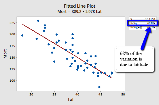
Let's revisit the skin cancer mortality example (Skin Cancer Data). Any statistical software that performs a simple linear regression analysis will report the r-squared value for you. It appears in two places in Minitab's output, namely on the fitted line plot:

and in the standard regression analysis output.
Analysis of Variance
| Source | DF | Adj SS | Adj MS | F-Value | P-Value |
|---|---|---|---|---|---|
| Regression | 1 | 36464 | 36464.2 | 99.80 | 0.000 |
| Lat | 1 | 36464 | 36464.2 | 99.80 | 0.000 |
| Error | 47 | 17173 | 365.4 | ||
| Lack-of-Fit | 30 | 12863 | 428.8 | 1.69 | 0.128 |
| Pure Error | 17 | 4310 | 253.6 | ||
| Total | 48 | 53637 |
Model Summary
| S | R-sq | R-sq (adj) | R-sq (pred) |
|---|---|---|---|
| 19.1150 | 67.98% | 67.30% | 65.12% |
We can say that 68% (shaded area above) of the variation in the skin cancer mortality rate is reduced by taking into account latitude. Or, we can say — with knowledge of what it really means — that 68% of the variation in skin cancer mortality is due to or explained by latitude.