Example 5-4: Pastry Sweetness Data Section

A designed experiment is done to assess how the moisture content and sweetness of a pastry product affect a taster’s rating of the product (Pastry dataset). In a designed experiment, the eight possible combinations of four moisture levels and two sweetness levels are studied. Two pastries are prepared and rated for each of the eight combinations, so the total sample size is n = 16. The y-variable is the rating of the pastry. The two x-variables are moisture and sweetness. The values (and sample sizes) of the x-variables were designed so that the x-variables were not correlated.
Correlation: Moisture, Sweetness
Pearson correlation of Moisture and Sweetness = 0.000
P-Value = 1.000
A plot of moisture versus sweetness (the two x-variables) is as follows:
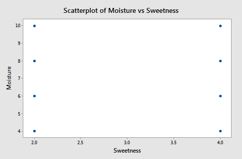
Notice that the points are on a rectangular grid so the correlation between the two variables is 0. (Please Note: we are not able to see that actually there are 2 observations at each location of the grid!)
The following figure shows how the two x-variables affect the pastry rating.
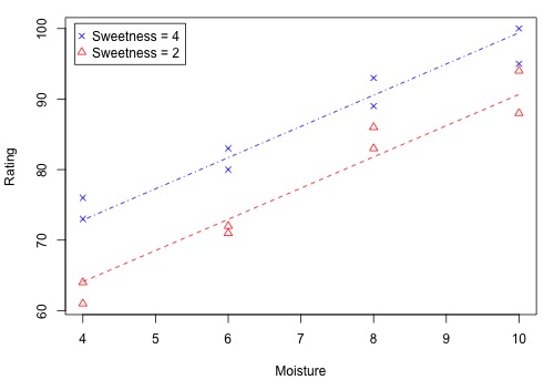
There is a linear relationship between rating and moisture and there is also a sweetness difference. The Minitab results given in the following output are for three different regressions - separate simple regressions for each x-variable and a multiple regression that incorporates both x-variables.
Regression Analysis: Rating versus Moisture
Analysis of Variance
| Source | DF | Adj SS | Adj MS | F-Value | P-value |
|---|---|---|---|---|---|
| Regression | 1 | 1566.45 | 1566.45 | 54.75 | 0.000 |
| Moisture | 1 | 166.45 | 1566.45 | 54.75 | 0.000 |
| Error | 14 | 400.55 | 28.61 | ||
| Lack-of-Fit | 2 | 15.05 | 7.52 | 0.23 | 0.795 |
| Pure Error | 12 | 385.50 | 32.13 | ||
| Total | 15 | 1967.00 |
Model Summary
| S | R-sq | R-sq(adj) | R-sq(pred) |
|---|---|---|---|
| 5.34890 | 79.64% | 78.18% | 72.71% |
Coefficients
| Term | Coef | SE Coef | T-Value | P-Value | VIF |
|---|---|---|---|---|---|
| Constant | 5077 | 4.39 | 11.55 | 0.000 | |
| Moisture | 4.425 | 0.598 | 7.40 | 0.000 | 1.00 |
Regression Equation
Rating = 50.77 + 4.425 Moisture
Regression Analysis: Rating versus Sweetness
Analysis of Variance
| Source | DF | Adj SS | Adj MS | F-Value | P-value |
|---|---|---|---|---|---|
| Regression | 1 | 306.3 | 306.3 | 2.58 | 0.130 |
| Sweetness | 1 | 306.3 | 306.3 | 2.58 | 0.130 |
| Error | 14 | 1660.8 | 118.6 | ||
| Total | 15 | 1967.0 |
Model Summary
| S | R-sq | R-sq(adj) | R-sq(pred) |
|---|---|---|---|
| 10.8915 | 15.57% | 9.54% | 0.00% |
Coefficients
| Term | Coef | SE Coef | T-Value | P-Value | VIF |
|---|---|---|---|---|---|
| Constant | 68.63 | 8.61 | 7.97 | 0.000 | |
| Sweetness | 4.38 | 2.72 | 1.61 | 0.130 | 1.00 |
Regression Equation
Rating = 68.63 + 4.38 Sweetness
Regression Analysis: Rating versus Moisture, Sweetness
Analysis of Variance
| Source | DF | Adj SS | Adj MS | F-Value | P-value |
|---|---|---|---|---|---|
| Regression | 2 | 1872.70 | 936.35 | 129.08 | 0.000 |
| Moisture | 1 | 1566.45 | 1566.45 | 215.95 | 0.000 |
| Sweetness | 1 | 306.25 | 306.25 | 42.22 | 0.000 |
| Error | 13 | 94.30 | 7.25 | ||
| Lack-of-Fit | 5 | 37.30 | 7.46 | 1.05 | 0.453 |
| 857.00 | 7.13 | ||||
| Total | 15 | 1967.00 |
Model Summary
| S | R-sq | R-sq(adj) | R-sq(pred) |
|---|---|---|---|
| 2.69330 | 95.21% | 94.47% | 92.46% |
Coefficients
| Term | Coef | SE Coef | T-Value | P-Value | VIF |
|---|---|---|---|---|---|
| Constant | 37.65 | 3.00 | 12.57 | 0.000 | |
| Moisture | 4.425 | 0.301 | 14.70 | 0.000 | 1.00 |
| Sweetness | 4.375 | 0.673 | 6.50 | 0.000 | 1.00 |
Regression Equation
Rating = 37.65 + 4.425 Moisture + 4.375 Sweetness
There are three important features to notice in the results:
-
The sample coefficient that multiplies Moisture is 4.425 in both the simple and the multiple regression. The sample coefficient that multiplies Sweetness is 4.375 in both the simple and the multiple regression. This result does not generally occur; the only reason that it does, in this case, is that Moisture and Sweetness are not correlated, so the estimated slopes are independent of each other. For most observational studies, predictors are typically correlated and estimated slopes in a multiple linear regression model do not match the corresponding slope estimates in simple linear regression models.
-
The \(R^{2}\) for the multiple regression, 95.21%, is the sum of the \(R^{2}\) values for the simple regressions (79.64% and 15.57%). Again, this will only happen when we have uncorrelated x-variables.
-
The variable Sweetness is not statistically significant in the simple regression (p = 0.130), but it is in the multiple regression. This is a benefit of doing a multiple regression. By putting both variables into the equation, we have greatly reduced the standard deviation of the residuals (notice the S values). This in turn reduces the standard errors of the coefficients, leading to greater t-values and smaller p-values.
(Data source: Applied Regression Models, (4th edition), Kutner, Neter, and Nachtsheim).
Example 5-5: Female Stat Students Section
The data are from n = 214 females in statistics classes at the University of California at Davis (Stat Females dataset). The variables are y = student’s self-reported height, \(x_{1}\) = student’s guess at her mother’s height, and \(x_{2}\) = student’s guess at her father’s height. All heights are in inches. The scatterplots below are of each student’s height versus the mother’s height and the student’s height against the father’s height.
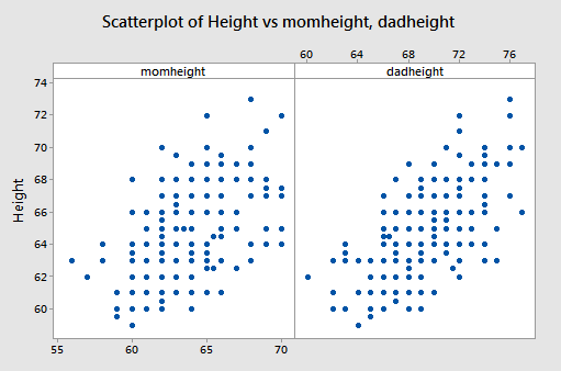
Both show a moderate positive association with a straight-line pattern and no notable outliers.
Interpretations
The first two lines of the Minitab output show that the sample multiple regression equations is predicted student height = 18.55 + 0.3035 × mother’s height + 0.3879 × father’s height:
Regression Analysis: Height versus momheight, dadheight
Analysis of Variance
| Source | DF | Adj SS | Adj MS | F-Value | P-value |
|---|---|---|---|---|---|
| Regression | 2 | 666.1 | 333.074 | 80.73 | 0.000 |
| momheight | 1 | 128.1 | 128.117 | 31.05 | 0.000 |
| dadheight | 1 | 278.5 | 278.488 | 67.50 | 0.000 |
| Error | 211 | 870.5 | 4.126 | ||
| Lack-of-Fit | 101 | 446.3 | 4.419 | 1.15 | 0.242 |
| Pure Error | 110 | 424.2 | 3.857 | ||
| Total | 213 | 1536.6 |
Model Summary
| S | R-sq | R-sq(adj) | R-sq(pred) |
|---|---|---|---|
| 2.03115 | 43.35% | 42.81% | 41.58% |
Coefficients
| Term | Coef | SE Coef | T-Value | P-Value | VIF |
|---|---|---|---|---|---|
| Constant | 18.55 | 3.69 | 5.02 | 0.000 | |
| momheight | 0.3035 | 0.0545 | 5.57 | 0.000 | 1.19 |
| dadheight | 0.3879 | 0.0472 | 8.22 | 0.000 | 1.19 |
Regression Equation
Rating = 18.55 + 0.3035 momheight + 0.3879 dadheight
To use this equation for prediction, we substitute specified values for the two parents’ heights.
We can interpret the “slopes” in the same way that we do for a simple linear regression model but we have to add the constraint that values of other variables remain constant. For example:
– When the father’s height is held constant, the average student height increases by 0.3035 inches for each one-inch increase in the mother’s height.
– When the mother’s height is held constant, the average student height increases by 0.3879 inches for each one-inch increase in the father’s height.
- The p-values given for the two x-variables tell us that student height is significantly related to each.
- The value of \(R^{2}\) = 43.35% means that the model (the two x-variables) explains 43.35% of the observed variation in student heights.
- The value S = 2.03115 is the estimated standard deviation of the regression errors. Roughly, it is the average absolute size of a residual.
Residual Plots
Just as in simple regression, we can use a plot of residuals versus fits to evaluate the validity of assumptions. The residual plot for these data is shown in the following figure:
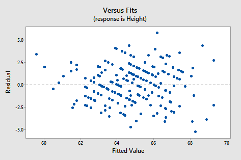
It looks about as it should - a random horizontal band of points. Other residual analyses can be done exactly as we did for simple regression. For instance, we might wish to examine a normal probability plot of the residuals. Additional plots to consider are plots of residuals versus each x-variable separately. This might help us identify sources of curvature or non-constant variance.
Example 5-6: Hospital Data Section

Data from n = 113 hospitals in the United States are used to assess factors related to the likelihood that a hospital patient acquires an infection while hospitalized. The variables here are y = infection risk, \(x_{1}\) = average length of patient stay, \(x_{2}\) = average patient age, \(x_{3}\) = measure of how many x-rays are given in the hospital (Hospital Infection dataset). The Minitab output is as follows:
Coefficients
| Term | Coef | SE Coef | T-Value | P-Value | VIF |
|---|---|---|---|---|---|
| Constant | 1.00 | 1.31 | 0.76 | 0.448 | |
| Stay | 0.3082 | 0.0594 | 5.19 | 0.000 | 1.23 |
| Age | -0.0230 | 0.0235 | -0.98 | 0.330 | 1.05 |
| Xray | 0.01966 | 0.00576 | 3.41 | 0.001 | 1.18 |
Regression Equation
InfctRsk = 1.00 + 0.3082 Stay - 0.0230 Age + 0.01966 Xray
Interpretations for this example include:
- The p-value for testing the coefficient that multiplies Age is 0.330. Thus we cannot reject the null hypothesis \(H_0 \colon \beta_{2}\) = 0. The variable Age is not a useful predictor within this model that includes Stay and Xrays.
- For the variables Stay and X-rays, the p-values for testing their coefficients are at a statistically significant level so both are useful predictors of infection risk (within the context of this model!).
- We usually don’t worry about the p-value for Constant. It has to do with the “intercept” of the model and seldom has any practical meaning. It also doesn’t give information about how changing an x-variable might change y-values.
(Data source: Applied Regression Models, (4th edition), Kutner, Neter, and Nachtsheim).
Example 5-7: Physiological Measurements Data Section
For a sample of n = 20 individuals, we have measurements of y = body fat, \(x_{1}\) = triceps skinfold thickness, \(x_{2}\) = thigh circumference, and \(x_{3}\) = midarm circumference (Body Fat dataset). Minitab results for the sample coefficients, MSE (highlighted), and \(\left(X^{T} X \right)^{−1}\) are given below:
Regression Analysis: Bodyfat versus Triceps, Thigh, Midarm
Analysis of Variance
| Source | DF | Adj SS | Adj MS | F-Value | P-Value |
|---|---|---|---|---|---|
| Regression | 3 | 396.985 | 132.328 | 21.52 | 0.000 |
| Triceps | 1 | 12.705 | 12.705 | 2.07 | 0.170 |
| Thigh | 1 | 7.529 | 7.529 | 1.22 | 0.285 |
| Midarm | 1 | 11.546 | 11.546 | 1.88 | 0.190 |
| Error | 16 | 98.405 | 6.150 | ||
| Total | 19 | 495.390 |
Model Summary
| S | R-sq | R-sq(adj) | R-sq(pred) |
|---|---|---|---|
| 2.47998 | 80.14% | 76.41% | 67.55% |
Coefficients
| Predictor | Coef | SE Coef | T-Value | P-Value | VIF |
|---|---|---|---|---|---|
| Constant | 117.1 | 99.8 | 1.17 | 0.258 | |
| Triceps | 4.33 | 3.02 | 1.44 | 0.170 | 708.84 |
| Thigh | -2.86 | 2.58 | -1.11 | 0.285 | 564.34 |
| Midarm | -2.19 | 1.60 | -1.37 | 0.190 | 104.61 |
Regression Equation
Bodyfat 117.1 + 4.33 Triceps - 2.86 Thigh - 2.19 Midarm
\(\left(X^{T} X \right)^{−1}\) - (calculated manually, see note below)
| Body Fat Calculations | |||
|---|---|---|---|
| 1618.87 | 48.8103 | -41.8487 | -25.7988 |
| 48.81 | 1.4785 | -1.2648 | -0.7785 |
| -41.85 | -1.2648 | 1.0840 | 0.6658 |
| -25.80 | -0.7785 | 0.6658 | 0.4139 |
The variance-covariance matrix of the sample coefficients is found by multiplying each element in \(\left(X^{T} X \right)^{−1}\) by MSE. Common notation for the resulting matrix is either \(s^{2}\)(b) or \(se^{2}\)(b). Thus, the standard errors of the coefficients given in the Minitab output can be calculated as follows:
- Var(\(b_{0}\)) = (6.15031)(1618.87) = 9956.55, so se(\(b_{0}\)) = \(\sqrt{9956.55}\) = 99.782.
- Var(\(b_{1}\)) = (6.15031)(1.4785) = 9.0932, so se(\(b_{1}\)) = \(\sqrt{9.0932}\) = 3.016.
- Var(\(b_{2}\)) = (6.15031)(1.0840) = 6.6669, so se(\(b_{2}\)) = \(\sqrt{6.6669}\) = 2.582.
- Var(\(b_{3}\)) = (6.15031)(0.4139) = 2.54561, so se(\(b_{3}\)) = \(\sqrt{2.54561}\) = 1.595.
As an example of covariance and correlation between two coefficients, we consider \(b_{1 }\)and \(b_{2}\).
- Cov(\(b_{1}\), \(b_{2}\)) = (6.15031)(−1.2648) = −7.7789. The value -1.2648 is in the second row and third column of \(\left(X^{T} X \right)^{−1}\). (Keep in mind that the first row and first column give information about \(b_0\), so the second row has information about \(b_{1}\), and so on.)
- Corr(\(b_{1}\), \(b_{2}\)) = covariance divided by product of standard errors = −7.7789 / (3.016 × 2.582) = −0.999.
The extremely high correlation between these two sample coefficient estimates results from a high correlation between the Triceps and Thigh variables. The consequence is that it is difficult to separate the individual effects of these two variables.
If all x-variables are uncorrelated with each other, then all covariances between pairs of sample coefficients that multiply x-variables will equal 0. This means that the estimate of one beta is not affected by the presence of the other x-variables. Many experiments are designed to achieve this property. With observational data, however, we’ll most likely not have this happen.
(Data source: Applied Regression Models, (4th edition), Kutner, Neter, and Nachtsheim).