In this section, we learn how to build and use a model by transforming both the response y and the predictor x. You might have to do this when everything seems wrong — when the regression function is not linear and the error terms are not normal and have unequal variances. In general (although not always!):
- Transforming the y values corrects problems with the error terms (and may help the non-linearity).
- Transforming the x values primarily corrects the non-linearity.
Again, keep in mind that although we're focussing on a simple linear regression model here, the essential ideas apply more generally to multiple linear regression models too.
As before, let's learn about transforming both the x and y values by way of an example.
Example 9-3: Short Leaf Section
Building the model
Many different interest groups — such as the lumber industry, ecologists, and foresters — benefit from being able to predict the volume of a tree just by knowing its diameter. One classic data set (Short Leaf data) — reported by C. Bruce and F. X. Schumacher in 1935 — concerned the diameter (x, in inches) and volume (y, in cubic feet) of n = 70 shortleaf pines. Let's use the data set to learn not only about the relationship between the diameter and volume of shortleaf pines, but also about the benefits of simultaneously transforming both the response y and the predictor x.
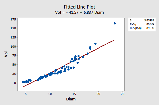
Although the \(r^{2}\) value is quite high (89.3%), the fitted line plot suggests that the relationship between tree volume and tree diameter is not linear:
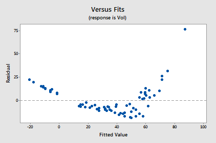
The residuals vs. fits plot also suggests that the relationship is not linear:
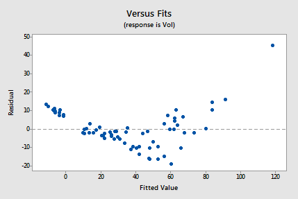
Because the lack of linearity dominates the plot, we can not use the plot to evaluate whether the error variances are equal. We have to fix the non-linearity problem before we can assess the assumption of equal variances.
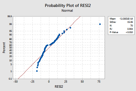
The normal probability plot suggests that the error terms are not normal. The plot is not quite linear and the Ryan-Joiner P-value is small. There is sufficient evidence to conclude that the error terms are not normally distributed:
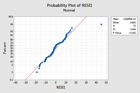
The plot actually has the classical appearance of residuals that are predominantly normal but have one outlier. This illustrates how a data point can be deemed an "outlier" just because of poor model fit.
In summary, it appears as if the relationship between tree diameter and volume is not linear. Furthermore, it appears as if the error terms are not normally distributed.
Let's see if we get anywhere by transforming only the x values. In particular, let's take the natural logarithm of the tree diameters to obtain the new predictor x = lnDiam:
| Diameter | Volume | lnDiam |
|---|---|---|
| 4.4 | 2.0 | 1.48160 |
| 4.6 | 2.2 | 1.52606 |
| 5.0 | 3.0 | 1.60944 |
| 5.1 | 4.3 | 1.62924 |
| 5.1 | 3.0 | 1.62924 |
| 5.2 | 2.9 | 1.64866 |
| 5.2 | 3.5 | 1.64866 |
| 5.5 | 3.4 | 1.70475 |
| 5.5 | 5.0 | 1.70475 |
| 5.6 | 7.2 | 1.72277 |
| 5.9 | 6.4 | 1.77495 |
| 5.9 | 5.6 | 1.77495 |
| 7.5 | 7.7 | 2.01490 |
| 7.6 | 10.3 | 2.02815 |
|
… and so on …
|
||
For example, ln(5.0) = 1.60944 and ln(7.6) = 2.02815. How well does transforming only the x values work? Not very!
The fitted line plot with y = volume as the response and x = lnDiam as the predictor suggests that the relationship is still not linear:
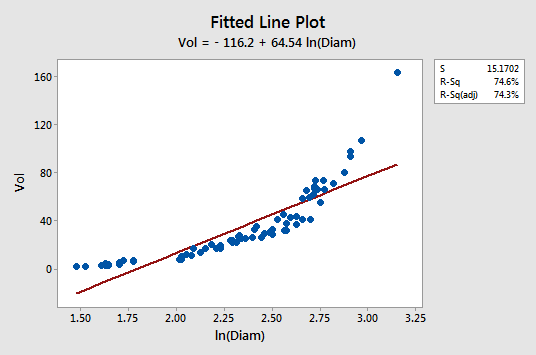
Transforming only the x values didn't change the non-linearity at all. The residuals vs. fits plot also still suggests a non-linear relationship ...
... and there is little improvement in the normality of the error terms:
The pattern is not linear and the Ryan-Joiner P-value is small. There is sufficient evidence to conclude that the error terms are not normally distributed.
So, transforming x alone didn't help much. Let's also try transforming the response (y) values. In particular, let's take the natural logarithm of the tree volumes to obtain the new response y = lnVol:
| Diameter | Volume | lnDiam | lnVol |
|---|---|---|---|
| 4.4 | 2.0 | 1.48160 | 0.69315 |
| 4.6 | 2.2 | 1.52606 | 0.78846 |
| 5.0 | 3.0 | 1.60944 | 1.09861 |
| 5.1 | 4.3 | 1.62924 | 1.45862 |
| 5.1 | 3.0 | 1.62924 | 1.09861 |
| 5.2 | 2.9 | 1.64866 | 1.06471 |
| 5.2 | 3.5 | 1.64866 | 1.25276 |
| 5.5 | 3.4 | 1.70475 | 1.22378 |
| 5.5 | 5.0 | 1.70475 | 1.60944 |
| 5.6 | 7.2 | 1.72277 | 1.97408 |
| 5.9 | 6.4 | 1.77495 | 1.85630 |
| 5.9 | 5.6 | 1.77495 | 1.72277 |
| 7.5 | 7.7 | 2.01490 | 2.04122 |
| 7.6 | 10.3 | 2.02815 | 2.33214 |
|
... and so on ...
|
|||
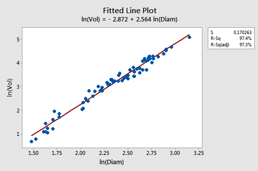
Let's see if transforming both the x and y values does it for us. Wow! The fitted line plot should give us hope! The relationship between the natural log of the diameter and the natural log of the volume looks linear and strong (\(r^{2} = 97.4\%)\colon\)
The residuals vs. fits plot provides yet more evidence of a linear relationship between lnVol and lnDiam:
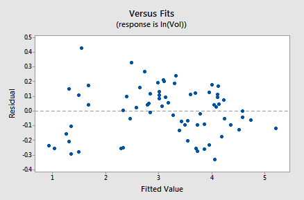
Generally, speaking the residuals bounce randomly around the residual = 0 line. You might be a little concerned that some "funneling" exists. If it does, it doesn't appear to be too severe, as the negative residuals do follow the desired horizontal band.
The normal probability plot has improved substantially:
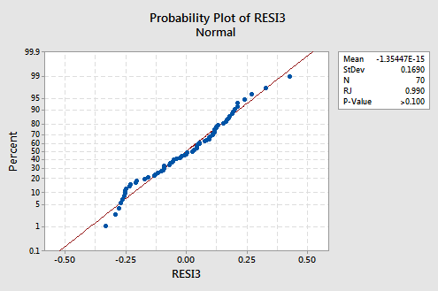
The trend is generally linear and the Ryan-Joiner P-value is large. There is insufficient evidence to conclude that the error terms are not normal.
In summary, it appears as if the model with the natural log of tree volume as the response and the natural log of tree diameter as the predictor works well. The relationship appears to be linear and the error terms appear independent and normally distributed with equal variances.
Using the Model
Let's now use our linear regression model for the shortleaf pine data — with y = lnVol as the response and x = lnDiam as the predictor — to answer four different research questions.
Research Question #1: What is the nature of the association between diameter and volume of shortleaf pines?
Again, to answer this research question, we just describe the nature of the relationship. That is, the natural logarithm of tree volume is positively linearly related to the natural logarithm of tree diameter. That is, as the natural log of tree diameters increases, the average natural logarithm of the tree volume also increases.
Research Question #2: Is there an association between the diameter and volume of shortleaf pines?
Again, in answering this research question, no modification to the standard procedure is necessary. We merely test the null hypothesis \(H_0\colon \beta_1 = 0\) using either the F-test or the equivalent t-test:
The regression equation is
\(\widehat{lnVol} = - 2.87 + 2.56 lnDiam\)
| Predictor | Coef | SE Coef | T | P |
|---|---|---|---|---|
| Constant | -2.8718 | 0.1215 | -23.63 | 0.000 |
| lnDiam | 2.56442 | 0.05120 | 50.09 | 0.000 |
| Model Summary | ||
|---|---|---|
| S = 0.1703 | R-Sq = 97.4% | R-Sq(adj) = 97.3% |
Analysis of Variance
| Source | DF | SS | MS | F | P |
|---|---|---|---|---|---|
| Regression | 1 | 72.734 | 72.734 | 2509.00 | 0.000 |
| Residual Error | 68 | 1.971 | 0.029 | ||
| Total | 69 | 74.706 |
As the Minitab output illustrates, the P-value is < 0.001. There is significant evidence at the 0.01 level to conclude that there is a linear association between the natural logarithm of tree volume and the natural logarithm of tree diameter.
Research Question #3: What is the "average" volume of all shortleaf pine trees that are 10" in diameter?
In answering this research question, if we are only interested in a point estimate, we put x = ln(10) = 2.30 into the estimated regression equation:
\(\widehat{lnVol} = - 2.87 + 2.56 lnDiam\)
to obtain:
\(\widehat{lnVol} = -2.87 + 2.56 × ln(10) = 3.025\)
That is, we estimate the average of the natural log of the volumes of all 10"-diameter shortleaf pines to be 3.025 log-cubic feet. Of course, this is not a very helpful conclusion. We have to take advantage of the fact, as we showed before, that the average of the natural log of the volumes approximately equals the natural log of the median of the volumes. Exponentiating both sides of the previous equation:
\(Vol = e^{ln \left(Vol \right)} = e^{3.025} = 20.6\) cubic feet
we estimate the median volume of all shortleaf pines with a 10" diameter to be 20.6 cubic feet. Helpful, but not sufficient! A 95% confidence interval for the average of the natural log of the volumes of all 10"-diameter shortleaf pines is:
Values of Predictions for New Observations
| New Obs | lnDiam |
|---|---|
| 1 | 2.30 |
Prediction Values for New Observations
| New | Fit | SE Fit | 95.0% CI | 95.0% PI |
|---|---|---|---|---|
| 1 | 3.030 | 0.0204 | (2.9922, 3.0738) | (2.6908, 3.3752) |
Exponentiating both endpoints of the interval, we get:
\(e^{2.9922} = 19.9\) and \(e^{3.0738} = 21.6\).
We can be 95% confident that the median volume of all shortleaf pines, 10" in diameter, is between 19.9 and 21.6 cubic feet.
Research Question #4: What is the expected change in volume for a two-fold increase in diameter?
Figuring out how to answer this research question also takes a little bit of work. The end result is:
- In general, the median changes by a factor of \(k^{\beta_1}\) for each k-fold increase in the predictor x.
- Therefore, the median changes by a factor of \(2^{\beta_1}\) for each two-fold increase in the predictor x.
- As always, we won't know the slope of the population line, \(\beta_1\). We have to use \(b_1\) to estimate it.
Again, you won't be required to duplicate the derivation, shown below, of this result, but it may help you to understand it and therefore remember it.
For the shortleaf pine data, the software output tells us that \(b_1 = 2.56442 \colon\)
| Predictor | Coef | SE Coef | T | P |
|---|---|---|---|---|
| Constant | -2.8718 | 0.1215 | -23.63 | 0.000 |
| lnDiam | 2.56442 | 0.05120 | 6.06 | 0.000 |
and therefore:
\(2^{b_1}=2^{2.56442}=5.92\)
The result tells us that the estimated median volume changes by a factor of 5.92 for each two-fold increase in diameter. For example, the median volume of a 20"-diameter tree is estimated to be 5.92 times the median volume of a 10" diameter tree. And, the median volume of a 10"-diameter tree is estimated to be 5.92 times the median volume of a 5"-diameter tree.
So far, we've only calculated a point estimate for the expected change. Of course, a 95% confidence interval for \(\beta_1\) is:
2.56442 ± 1.9955(0.05120) = (2.46, 2.67)
Because:
\(2^{2.46} = 5.50\) and \(2^{2.67} = 6.36\)
we can be 95% confident that the median volume will increase by a factor between 5.50 and 6.36 for each two-fold increase in diameter.
Example 9-4: Real Estate Air Conditioning Section
Recall the real estate dataset from Section 8.9: Real estate data, where
- \(Y =\) sale price of the home
- \(X_1 =\) square footage of home
- \(X_2 =\) whether the home has air conditioning or not.
The interaction model
\(y _ { i } = \beta _ { 0 } + \beta _ { 1 } x _ { i , 1 } + \beta _ { 2 } x _ { i , 2 } + \beta _ { 3 } x _ { i , 1 } x _ { i , 2 } + \varepsilon _ { i }\)
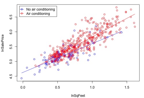
resulted in a residual plot with a megaphone pattern (i.e., an increasing variance problem). To remedy this, we'll try using log transformations for sale price and square footage (which are quite highly skewed). Now, Y = log(sale price), \(X_1 =\) log(home’s square foot area), and \(X_2 = 1\) if air conditioning present and 0 if not. After fitting the above interaction model with the transformed variables, the plot showing the regression lines is as follows:
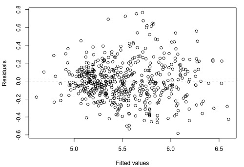
and the residual plot, which shows a vast improvement on the residual plot in Section 8.9, is as follows:
Try It!
Transforming x and y Section
Transforming both the predictor x and the response y to repair problems. Hospital administrators were interested in determining how hospitalization cost (y = cost) is related to the length of stay (x = los) in the hospital. The Hospital dataset contains the reimbursed hospital costs and associated lengths of stay for a sample of 33 elderly people.
-
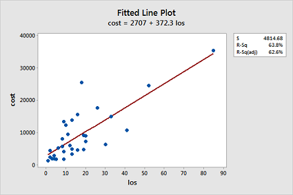
Fit a simple linear regression model using Minitab's fitted line plot command. (See Minitab Help: Creating a fitted line plot.) Does a linear function appear to fit the data well? Does the plot suggest any other potential problems with the model?
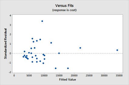
A linear function does not fit the data well since the data is clumped in the lower left corner and there appears to be an increasing variance problem:
-
Now, fit a simple linear regression model using Minitab's regression command. In doing so, store the standardized residuals (See Minitab Help: Storing residuals (and/or influence measures)), and request a (standardized) residuals vs. fits plot. (See Minitab Help: Creating residual plots.) Interpret the residuals vs. fits plot — which model assumption does it suggest is violated?
The residual plot confirms that the "equal variance" assumption is violated:
-
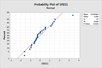
Test the normality of your stored standardized residuals using the Ryan-Joiner correlation test. (See Minitab Help: Conducting a Ryan-Joiner correlation test.) Does the test provide evidence that the residuals are not normally distributed?
The Ryan-Joiner p-value is less than 0.01, which suggests the normality assumption is violated too:
- Transform the response by taking the natural log of cost. You can use the calculator function. Select Calc >> Calculator... In the box labeled "Store result in variable", type lncost. In the box labeled Expression, use the calculator function "Natural log" or type LN('cost'). Select OK. The values of lncost should appear in the worksheet.
- Transform the predictor by taking the natural log of los. Again, you can use the calculator function. Select Calc >> Calculator... In the box labeled "Store result in variable", type lnlos. In the box labeled Expression, use the calculator function "Natural log" or type LN('los'). Select OK. The values of lnlos should appear in the worksheet.
-
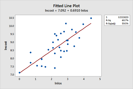
Now, fit a simple linear regression model using Minitab's fitted line plot command treating the response as lncost and the predictor as lnlos. (See Minitab Help: Creating a fitted line plot.) Does the transformation appear to have helped rectify the original problem with the model?
The transformations appear to have rectified the original problem with the model since the fitted line plot now looks ideal:
- Now, fit a simple linear regression model using Minitab's regression command treating the response as lncost and the predictor as lnlos. In doing so:
- Store the standardized residuals (See Minitab Help: Storing residuals (and/or influence measures)), and request a (standardized) residuals vs. fits plot. (See Minitab Help: Creating residual plots.)
-
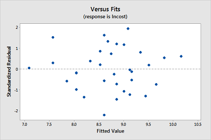
Interpret the residuals vs. fits plot — does the transformation appear to have helped rectify the original problem with the model?
The transformations appear to have rectified the original problem with the model since the residual plot also now looks ideal:
-
Test the normality of your new stored standardized residuals using the Ryan-Joiner correlation test. (See Minitab Help: Conducting a Ryan-Joiner correlation test.) Does the transformation appear to have helped rectify the non-normality of the residuals?
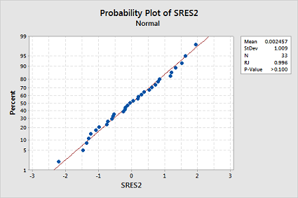
The transformations appear to have rectified the non-normality of the residuals since the Ryan-Joiner p-value is now greater than 0.1:
-
If you are satisfied that the "LINE" assumptions are met for the model based on the transformed values, you can now use the model to answer your research questions.
- Is there an association between hospitalization cost and length of stay?
- What is the expected change in hospitalization cost for each three-fold increase in length of stay?
The fitted model results are:
Model Summary
S R-sq R-sq(adj) R-sq(pred) 0.553820 60.75% 59.48% 56.65% Coefficients
Term Coef SE Coef T-Value P-Value VIF Constant 7.092 0.255 27.76 0.000 lnlos 0.6910 0.0998 6.93 0.000 1.00 - Since the p-value for lnlos is 0.000, there is significant evidence to conclude that there is a linear association between the natural logarithm of hospitalization cost and the natural logarithm of length of stay.
- Since \(3^{0.6910} = 2.14\), the estimated median cost changes by a factor of 2.14 for each three-fold increase in length of stay. A 95% confidence interval for the regression coefficient for lnlos is \(0.6910 \pm 2.03951(0.0998) = (0.487, 0.895)\), so a 95% confidence interval for this multiplicative change is \(\left(3^{0.487}, 3^{0.895} \right) = \left(1.71, 2.67 \right)\).