Exampe 10-4: Cement Data Section
Let's take a look at a few more examples to see how the best subsets and stepwise regression procedures assist us in identifying a final regression model.
Let's return one more time to the cement data example (Cement data set). Recall that the stepwise regression procedure:
Stepwise Selection of Terms
Candidate terms: x1, x2, x3, x4
| Terms | -----Step 1----- | -----Step 2----- | -----Step 3----- | -----Step 4----- | ||||
|---|---|---|---|---|---|---|---|---|
| Coef | P | Coef | P | Coef | P | Coef | P | |
| Constant | 117.57 | 103.10 | 71.6 | 52.58 | ||||
| x4 | -0.738 | 0.001 | -0.6140 | 0.000 | -0.237 | 0.205 | ||
| x1 | 1.440 | 0.000 | 1.452 | 0.000 | 1.468 | 0.000 | ||
| x2 | 0.416 | 0.052 | 0.6623 | 0.000 | ||||
| S | 8.96390 | 2.73427 | 2.30874 | 2.40634 | ||||
| R-sq | 67.45% | 97.25% | 98.23% | 97.44% | ||||
| R-sq(adj) | 64.50% | 96.70% | 97.64% | 97.44% | ||||
| R-sq(pred) | 56.03% | 95.54% | 96.86% | 96.54% | ||||
| Mallows' Cp | 138.73 | 5.50 | 3.02 | 2.68 | ||||
\(\alpha\) to enter =0.15, \(\alpha\) to remove 0.15
yielded the final stepwise model with y as the response and \(x_1\) and \(x_2\) as predictors.
The best subsets regression procedure:
Best Subsets Regressions: y versus x1, x2, x3, x4
Response is y
| Vars | R-Sq | R-Sq (adj) |
R-Sq (pred) |
Mallows Cp |
S | x | x | x | x |
|---|---|---|---|---|---|---|---|---|---|
| 1 | 2 | 3 | 4 | ||||||
| 1 | 67.5 | 64.5 | 56.0 | 138.7 | 8.9639 | X | |||
| 1 | 66.6 | 63.6 | 55.7 | 142.5 | 9.0771 | X | |||
| 2 | 97.9 | 97.4 | 96.5 | 2.7 | 2.4063 | X | X | ||
| 2 | 97.2 | 96.7 | 95.5 | 5.5 | 2.7343 | X | X | ||
| 3 | 98.2 | 97.6 | 96.9 | 3.0 | 2.3087 | X | X | X | |
| 3 | 98.2 | 97.6 | 96.7 | 3.0 | 2.3121 | X | X | X | |
| 4 | 98.2 | 97.4 | 95.9 | 5.0 | 2.4460 | X | X | X | X |
yields various models depending on the different criteria:
- Based on the \(R^{2} \text{-value}\) criterion, the "best" model is the model with the two predictors \(x_1\) and \(x_2\).
- Based on the adjusted \(R^{2} \text{-value}\) and MSE criteria, the "best" model is the model with the three predictors \(x_1\), \(x_2\), and \(x_4\).
- Based on the \(C_p\) criterion, there are three possible "best" models — the model containing \(x_1\) and \(x_2\); the model containing \(x_1\), \(x_2\) and \(x_3\); and the model containing \(x_1\), \(x_2\) and \(x_4\).
So, which model should we "go with"? That's where the final step — the refining step — comes into play. In the refining step, we evaluate each of the models identified by the best subsets and stepwise procedures to see if there is a reason to select one of the models over the other. This step may also involve adding interaction or quadratic terms, as well as transforming the response and/or predictors. And, certainly, when selecting a final model, don't forget why you are performing the research, to begin with — the reason may choose the model obviously.
Well, let's evaluate the three remaining candidate models. We don't have to go very far with the model containing the predictors \(x_1\), \(x_2\), and \(x_4\) :
Analysis of Variance: y versus x1, x2, x4
| Source | DF | Adj SS | Adj MS | F-Value | P-Value |
|---|---|---|---|---|---|
| Regression | 3 | 2667.79 | 889.263 | 166.83 | 0.000 |
| x1 | 1 | 820.91 | 820.907 | 154.01 | 0.000 |
| x2 | 1 | 26.79 | 26.789 | 5.03 | 0.052 |
| x4 | 1 | 9.93 | 9.932 | 1.86 | 0.205 |
| Error | 9 | 47.97 | 5.330 | ||
| Total | 12 | 2715.76 |
Model Summary
| S | R-sq | R-sq(adj) | R-sq(pred) |
|---|---|---|---|
| 2.30874 | 98.23% | 97.64% | 96.86% |
Coefficients
| Term | Coef | SE Coef | T-Value | P-Value | VIF |
|---|---|---|---|---|---|
| Constant | 71.6 | 14.1 | 5.07 | 0.001 | |
| x1 | 1.452 | 0.117 | 12.41 | 0.000 | 1.07 |
| x2 | 0.416 | 0.186 | 2.24 | 0.052 | 18.78 |
| x4 | -0.237 | 0.173 | -1.37 | 0.205 | 18.94 |
Regression Equaation
y = 71.6 + 1.452 x1 + 0.416 x2 - 0.237 x4
We'll learn more about multicollinearity in Lesson 12, but for now, all we need to know is that the variance inflation factors of 18.78 and 18.94 for \(x_2\) and \(x_4\) indicate that the model exhibits substantial multicollinearity. You may recall that the predictors \(x_2\) and \(x_4\) are strongly negatively correlated — indeed, r = -0.973.
While not perfect, the variance inflation factors for the model containing the predictors \(x_1\), \(x_2\), and \(x_3\):
Analysis of Variance: y versus x1, x2, x3
| Source | DF | Adj SS | Adj MS | F-Value | P-Value |
|---|---|---|---|---|---|
| Regression | 3 | 2667.65 | 889.22 | 166.34 | 0.000 |
| x1 | 1 | 367.33 | 367.33 | 68.72 | 0.000 |
| x2 | 1 | 1178.96 | 1178.96 | 220.55 | 0.000 |
| x3 | 1 | 9.79 | 9.79 | 1.83 | 0.209 |
| Error | 9 | 48.11 | 5.35 | ||
| Total | 12 | 2715.76 |
Model Summary
| S | R-sq | R-sq(adj) | R-sq(pred) |
|---|---|---|---|
| 2.31206 | 98.23% | 97.64% | 96.69% |
Coefficients
| Term | Coef | SE Coef | T-Value | P-Value | VIF |
|---|---|---|---|---|---|
| Constant | 48.19 | 3.91 | 12.32 | 0.000 | |
| x1 |
1.696 |
0.205 | 8.29 | 0.000 | 2.25 |
| x2 | 0.6569 | 0.0442 | 14.85 | 0.000 | 1.06 |
| x3 | 0.250 | 0.185 | 1.35 | 0.209 | 3.14 |
Regression Equation
y = 48.19 + 1.696 x1 + 0.6569 x2 + 0.250 x3
are much better (smaller) than the previous variance inflation factors. But, unless there is a good scientific reason to go with this larger model, it probably makes more sense to go with the smaller, simpler model containing just the two predictors \(x_1\) and \(x_2\):
Analysis of Variance: y versus x1, x2
| Source | DF | Adj SS | Adj MS | F-Value | P-Value |
|---|---|---|---|---|---|
| Regression | 2 | 2657.86 | 1328.93 | 229.50 | 0.000 |
| x1 | 1 | 848.43 | 848.43 | 146.52 | 0.000 |
| x2 | 1 | 1207.78 | 1207.78 | 208.58 | 0.000 |
| Error | 10 | 57.90 | 5.79 | ||
| Total | 12 | 2715.76 |
Model Summary
| S | R-sq | R-sq(adj) | R-sq(pred) |
|---|---|---|---|
| 2.40634 | 97.87% | 97.44% | 96.54% |
Coefficients
| Term | Coef | SE Coef | T-Value | P-Value | VIF |
|---|---|---|---|---|---|
| Constant | 52.58 | 2.29 | 23.00 | 0.000 | |
| x1 | 1.468 | 0.121 | 12.10 | 0.000 | 1.06 |
| x2 | 0.6623 | 0.0459 | 14.44 | 0.000 | 1.06 |
Regression Equation
y = 52.58 + 1.468 x1 + 0.6623 x2
For this model, the variance inflation factors are quite satisfactory (both 1.06), the adjusted \(R^{2} \text{-value}\) (97.44%) is large, and the residual analysis yields no concerns. That is, the residuals versus fits plot:
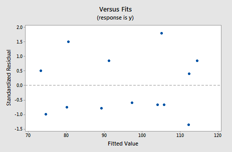
suggests that the relationship is indeed linear and that the variances of the error terms are constant. Furthermore, the normal probability plot:
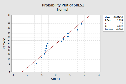
suggests that the error terms are normally distributed. The regression model with y as the response and \(x_1\) and \(x_2\) as the predictors has been evaluated fully and appears to be ready to answer the researcher's questions.
Example 10-5: IQ Size Section
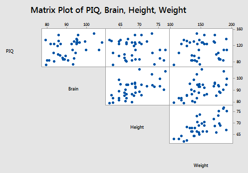
Let's return to the brain size and body size study, in which the researchers were interested in determining whether or not a person's brain size and body size are predictive of his or her intelligence. The researchers (Willerman, et al, 1991) collected the following IQ Size data on a sample of n = 38 college students:
- Response (y): Performance IQ scores (PIQ) from the revised Wechsler Adult Intelligence Scale. This variable served as the investigator's measure of the individual's intelligence.
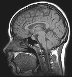
- Potential predictor (\(x_1\)): Brain size based on the count obtained from MRI scans (given as count/10,000).
- Potential predictor (\(x_2\)): Height in inches.
- Potential predictor (\(x_3\)): Weight in pounds.
A matrix plot of the resulting data looks like this:
The stepwise regression procedure:
Regression analysis: PIQ versus Brain, Height, Weight
Stepwise Selection of Terms
Candidate terms: Brain, Height, Weight
| Terms | --------Step 1-------- | --------Step 2-------- | ||
|---|---|---|---|---|
| Coef | P | Coef | P | |
| Constant | 4.7 | 111.3 | ||
| Brain | 1.177 | 0.019 | 2.061 | 0.001 |
| Height | -2.730 | 0.009 | ||
| S | 21.2115 | 19.5096 | ||
| R-sq | 14.27% | 29.49% | ||
| R-sq(adj) | 11.89% | 25.46% | ||
| R-sq(pred) | 4.60% | 17.63% | ||
| Mallows' Cp | 7.34 | 2.00 | ||
\(\alpha\) to enter =0.15, \(\alpha\) to remove 0.15
yielded the final stepwise model with PIQ as the response and Brain and Height as predictors. In this case, the best subsets regression procedure:
Best Subsets Regressions: PIQ versus Brain, Height, Weight
Response is PIQ
| Vars | R-Sq | R-Sq (adj) |
R-Sq (pred) |
Mallows Cp |
S | Brain | Height | Weight |
|---|---|---|---|---|---|---|---|---|
| 1 | 2 | 3 | ||||||
| 1 | 14.3 | 11.9 | 4.66 | 7.3 | 21.212 | X | ||
| 1 | 0.9 | 0.0 | 0.0 | 13.8 | 22.810 | X | ||
| 2 | 29.5 | 25.5 | 17.6 | 2.0 | 19.510 | X | X | |
| 2 | 19.3 | 14.6 | 5.9 | 6.9 | 20.878 | X | X | |
| 3 | 29.5 | 23.3 | 12.8 | 4.0 | 19.794 | X | X | X |
yields the same model regardless of the criterion used:
- Based on the \(R^{2} \text{-value}\) criterion, the "best" model is the model with the two predictors Brain and Height.
- Based on the adjusted \(R^{2} \text{-value}\) and MSE criteria, the "best" model is the model with the two predictors of Brain and Height.
- Based on the \(C_p\) criterion, the "best" model is the model with the two predictors Brain and Height.
Well, at least, in this case, we have only one model to evaluate further:
Analysis of Variance: PIQ versus Brain, Height
| Source | DF | Adj SS | Adj MS | F-Value | P-Value |
|---|---|---|---|---|---|
| Regression | 2 | 5573 | 2786.4 | 7.32 | 0.002 |
| Brain | 1 | 5409 | 5408.8 | 14.21 | 0.001 |
| Height | 1 | 2876 | 2875.6 | 7.56 | 0.009 |
| Error | 35 | 13322 | 380.6 | ||
| Total | 37 | 18895 |
Model Summary
| S | R-sq | R-sq(adj) | R-sq(pred) |
|---|---|---|---|
| 19.5069 | 29.49% | 25.46% | 17.63% |
Coefficients
| Term | Coef | SE Coef | T-Value | P-Value | VIF |
|---|---|---|---|---|---|
| Constant | 111.3 | 55.9 | 1.99 | 0.054 | |
| Brain |
2.061 |
0.547 | 3.77 | 0.001 | 1.53 |
| Height | -2.730 | 0.993 | -2.75 | 0.009 | 1.53 |
Regression Equation
PIQ = 11.3 + 2.061 Brain - 2.730 Height
For this model, the variance inflation factors are quite satisfactory (both 1.53), the adjusted \(R^{2} \text{-value}\) (25.46%) is not great but can't get any better with these data, and the residual analysis yields no concerns. That is, the residuals versus fits plot:
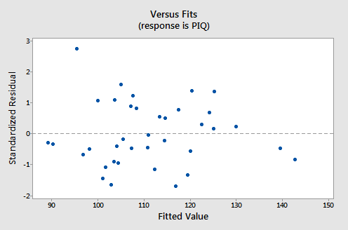
suggests that the relationship is indeed linear and that the variances of the error terms are constant. The researcher might want to investigate the one outlier, however. The normal probability plot:
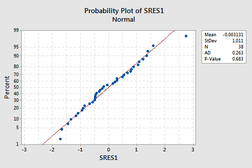
suggests that the error terms are normally distributed. The regression model with PIQ as the response and Brain and Height as the predictors has been evaluated fully and appears to be ready to answer the researchers' questions.
Example 10-6: Blood Pressure Section
Let's return to the blood pressure study in which we observed the following data (Blood Pressure data) on 20 individuals with hypertension:
- blood pressure (y = BP, in mm Hg)
- age (\(x_1\) = Age, in years)
- weight (\(x_2\) = Weight, in kg)
- body surface area (\(x_3\) = BSA, in sq m)
- duration of hypertension (\(x_4\) = Dur, in years)
- basal pulse (\(x_5\) = Pulse, in beats per minute)
- stress index (\(x_6\) = Stress)
The researchers were interested in determining if a relationship exists between blood pressure and age, weight, body surface area, duration, pulse rate and/or stress level.
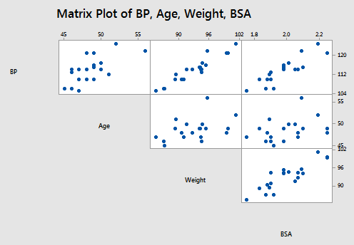
The matrix plot of BP, Age, Weight, and BSA looks like this:
and the matrix plot of BP, Dur, Pulse, and Stress looks like this:

The stepwise regression procedure:
Regressions Analysis: BP versus Age, Weight, BSA, Dur, Pulse, Stress
Stepwise Selection of Terms
Candidate terms: x1, x2, x3, x4
| Terms | -----Step 1----- | -----Step 2----- | -----Step 3----- | |||
|---|---|---|---|---|---|---|
| Coef | P | Coef | P | Coef | P | |
| Constant | 2.21 | -16.58 | -13.67 | |||
| Weight | 1.2009 | 0.000 | 1.0330 | 0.000 | 0.9058 | 0.000 |
| Age | 0.7083 | 0.000 | 0.7016 | 0.000 | ||
| BSA | 4.63 | 0.008 | ||||
| S | 1.74050 | 0.532692 | 0.437046 | |||
| R-sq | 90.26% | 99.14% | 99.455 | |||
| R-sq(adj) | 89.72% | 99.045 | 99.35% | |||
| R-sq(pred) | 88.53% | 98.89% | 99.22% | |||
| Mallows' Cp | 312.81 | 15.09 | 6.43 | |||
\(\alpha\) to enter =0.15, \(\alpha\) to remove 0.15
yielded the final stepwise model with PIQ as the response and Age, Weight, and BSA (body surface area) as predictors. The best subsets regression procedure:
Best Subsets Regressions: BP versus Age, Weight, BSA, Dur, Pulse, Stress
Response is BP
| Vars | R-Sq | R-Sq (adj) |
R-Sq (pred) |
Mallows Cp |
S | Age | Weight | BSA | Dur | Pulse | Stress |
|---|---|---|---|---|---|---|---|---|---|---|---|
| 1 | 90.3 | 89.7 | 88.5 | 312.8 | 1.7405 | X | |||||
| 1 | 75.0 | 73.6 | 69.5 | 829.1 | 2.7903 | X | |||||
| 2 | 99.1 | 99.0 | 98.9 | 15.1 | 0.53269 | X | X | ||||
| 2 | 92.0 | 91.0 | 89.3 | 256.6 | 1.6246 | X | X | ||||
| 3 | 99.5 | 99.4 | 99.2 | 6.4 | 0.43705 | X | X | X | |||
| 3 | 99.2 | 99.1 | 98.8 | 14.1 | 0.52012 | X | X | X | |||
| 4 | 99.5 | 99.4 | 99.2 | 6.4 | 0.42591 | X | X | X | X | ||
| 4 | 99.5 | 99.4 | 99.1 | 7.1 | 0.43500 | X | X | X | X | ||
| 5 | 99.6 | 99.4 | 99.1 | 7.0 | 0.42142 | X | X | X | X | X | |
| 5 | 99.5 | 99.4 | 99.2 | 7.7 | 0.43078 | X | X | X | X | X | |
| 6 | 99.6 | 99.4 | 99.1 | 7.0 | 0.40723 | X | X | X | X | X | X |
yields various models depending on the different criteria:
- Based on the \(R^{2} \text{-value}\) criterion, the "best" model is the model with the two predictors Age and Weight.
- Based on the adjusted \(R^{2} \text{-value}\) and MSE criteria, the "best" model is the model with all six of the predictors — Age, Weight, BSA, Duration, Pulse, and Stress — in the model. However, one could easily argue that any number of sub-models are also satisfactory based on these criteria — such as the model containing Age, Weight, BSA, and Duration.
- Based on the \(C_p\) criterion, a couple of models stand out — namely the model containing Age, Weight, and BSA; and the model containing Age, Weight, BSA, and Duration.
Incidentally, did you notice how large some of the \(C_p\) values are for some of the models? Those are the models that you should be concerned about exhibiting substantial bias. Don't worry too much about \(C_p\) values that are only slightly larger than p.
Here's a case in which I might argue for thinking practically over thinking statistically. There appears to be nothing substantially wrong with the two-predictor model containing Age and Weight:
Analysis of Variance: BP versus Age, Weight
| Source | DF | Adj SS | Adj MS | F-Value | P-Value |
|---|---|---|---|---|---|
| Regression | 2 | 55.176 | 277.588 | 978.25 | 0.000 |
| Age | 1 | 49.704 | 49.704 | 175.16 | 0.000 |
| Weight | 1 | 311.910 | 311.910 | 1099.20 | 0.000 |
| Error | 17 | 4.824 | 0.284 | ||
| Lack-of-Fit | 16 | 4.324 | 0.270 | 0.54 | 0.807 |
| Pure Error | 1 | 0.500 | 0.500 | ||
| Total | 19 | 590.000 |
Model Summary
| S | R-sq | R-sq(adj) | R-sq(pred) |
|---|---|---|---|
| 0.532692 | 99.14% | 99.04% | 98.89% |
Coefficients
| Term | Coef | SE Coef | T-Value | P-Value | VIF |
|---|---|---|---|---|---|
| Constant | -16.58 | 3.01 | -5.51 | 0.000 | |
| Age |
0.7083 |
0.0535 | 13.23 | 0.000 | 1.20 |
| Weight | 1.0330 | 0.0312 | 33.15 | 0.000 | 1.20 |
Regression Equation
BP = -16.58 + 0.7083 Age + 1.0330 Weight
For this model, the variance inflation factors are quite satisfactory (both 1.20), the adjusted \(R^{2} \text{-value}\) (99.04%) can't get much better, and the residual analysis yields no concerns. That is, the residuals versus fits plot:
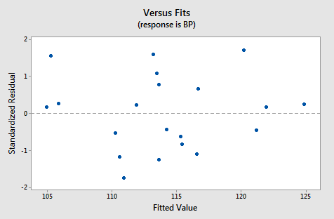
is just right, suggesting that the relationship is indeed linear and that the variances of the error terms are constant. The normal probability plot:
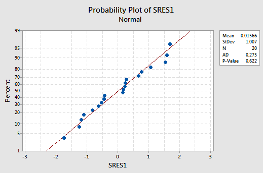
suggests that the error terms are normally distributed.
Now, why might I prefer this model over the other legitimate contenders? It all comes down to simplicity! What's your age? What's your weight? Perhaps more than 90% of you know the answer to those two simple questions. But, now what is your body surface area? And, how long have you had hypertension? Answers to these last two questions are almost certainly less immediate for most (all?) people. Now, the researchers might have good arguments for why we should instead use the larger, more complex models. If that's the case, fine. But, if not, it is almost always best to go with the simpler model. And, certainly, the model containing only Age and Weight is simpler than the other viable models.
The following video will walk through this example in Minitab.