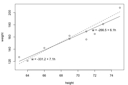
Since we are interested in summarizing the trend between two quantitative variables, the natural question arises — "what is the best fitting line?" At some point in your education, you were probably shown a scatter plot of (x, y) data and were asked to draw the "most appropriate" line through the data. Even if you weren't, you can try it now on a set of heights (x) and weights (y) of 10 students, (Student Height and Weight Dataset). Looking at the plot below, which line — the solid line or the dashed line — do you think best summarizes the trend between height and weight?
Hold on to your answer! In order to examine which of the two lines is a better fit, we first need to introduce some common notation:
- \(y_i\) denotes the observed response for experimental unit i
- \(x_i\) denotes the predictor value for experimental unit i
- \(\hat{y}_i\) is the predicted response (or fitted value) for experimental unit i
Then, the equation for the best-fitting line is:
\(\hat{y}_i=b_0+b_1x_i\)
Incidentally, recall that an "experimental unit" is the object or person on which the measurement is made. In our height and weight example, the experimental units are students.
Let's try out the notation on our example with the trend summarized by the line \(\hat{w} = -266.53 + 6.1376 h\).
The first data point in the list indicates that student 1 is 63 inches tall and weighs 127 pounds. That is, \(x_{1} = 63\) and \(y_{1} = 127\) . Do you see this point in the plot? If we know this student's height but not his or her weight, we could use the equation of the line to predict his or her weight. We'd predict the student's weight to be -266.53 + 6.1376(63) or 120.1 pounds. That is, \(\hat{y}_1 = 120.1\). Clearly, our prediction wouldn't be perfectly correct — it has some "prediction error" (or "residual error"). In fact, the size of its prediction error is 127-120.1 or 6.9 pounds.
You might want to roll your cursor over each of the 10 data points to make sure you understand the notation used to keep track of the predictor values, the observed responses, and the predicted responses:
i | \(x_i\) | \(y_i\) | \(\hat{y}_i\) |
|---|---|---|---|
1 | 63 | 127 | 120.1 |
2 | 64 | 121 | 126.3 |
3 | 66 | 142 | 138.5 |
4 | 69 | 157 | 157.0 |
5 | 69 | 162 | 157.0 |
6 | 71 | 156 | 169.2 |
7 | 71 | 169 | 169.2 |
8 | 72 | 165 | 175.4 |
9 | 73 | 181 | 181.5 |
10 | 75 | 208 | 193.8 |
As you can see, the size of the prediction error depends on the data point. If we didn't know the weight of student 5, the equation of the line would predict his or her weight to be -266.53 + 6.1376(69) or 157 pounds. The size of the prediction error here is 162-157 or 5 pounds.
In general, when we use \(\hat{y}_i=b_0+b_1x_i\) to predict the actual response \(y_i\), we make a prediction error (or residual error) of size:
\(e_i=y_i-\hat{y}_i\)
A line that fits the data "best" will be one for which the n prediction errors — one for each observed data point — are as small as possible in some overall sense. One way to achieve this goal is to invoke the "least squares criterion," which says to "minimize the sum of the squared prediction errors." That is:
- The equation of the best fitting line is: \(\hat{y}_i=b_0+b_1x_i\)
- We just need to find the values \(b_{0}\) and \(b_{1}\) which make the sum of the squared prediction errors the smallest they can be.
- That is, we need to find the values \(b_{0}\) and \(b_{1}\) that minimize:
\(Q=\sum_{i=1}^{n}(y_i-\hat{y}_i)^2\)
Here's how you might think about this quantity Q:
- The quantity \(e_i=y_i-\hat{y}_i\) is the prediction error for data point i.
- The quantity \(e_i^2=(y_i-\hat{y}_i)^2\) is the squared prediction error for data point i.
- And, the symbol \(\sum_{i=1}^{n}\) tells us to add up the squared prediction errors for all n data points.
Incidentally, if we didn't square the prediction error \(e_i=y_i-\hat{y}_i\) to get \(e_i^2=(y_i-\hat{y}_i)^2\), the positive and negative prediction errors would cancel each other out when summed, always yielding 0.
Now, being familiar with the least squares criterion, let's take a fresh look at our plot again. In light of the least squares criterion, which line do you now think is the best-fitting line?
Let's see how you did! The following two side-by-side tables illustrate the implementation of the least squares criterion for the two lines up for consideration — the dashed line and the solid line.
\(\hat{w} = -331.2 + 7.1 h\) (the dashed line)
i | \(x_i\) | \(y_i\) | \(\hat{y}_i\) | \((y_i-\hat{y}_i)\) | \((y_i-\hat{y}_i)^2\) |
|---|---|---|---|---|---|
1 | 63 | 127 | 116.1 | 10.9 | 118.81 |
2 | 64 | 121 | 123.2 | -2.2 | 4.84 |
3 | 66 | 142 | 137.4 | 4.6 | 21.16 |
4 | 69 | 157 | 158.7 | -1.7 | 2.89 |
5 | 69 | 162 | 158.7 | 3.3 | 10.89 |
6 | 71 | 156 | 172.9 | -16.9 | 285.61 |
7 | 71 | 169 | 172.9 | -3.9 | 15.21 |
8 | 72 | 165 | 180.0 | -15.0 | 225.00 |
9 | 73 | 181 | 187.1 | -6.1 | 37.21 |
10 | 75 | 208 | 201.3 | 6.7 | 44.89 |
______ 766.5 |
\(\hat{w}= -266.53 + 6.1376 h\) (the solid line)
i | \(x_i\) | \(y_i\) | \(\hat{y}_i\) | \((y_i-\hat{y}_i)\) | \((y_i-\hat{y}_i)^2\) |
|---|---|---|---|---|---|
1 | 63 | 127 | 120.139 | 6.8612 | 47.076 |
2 | 64 | 121 | 126.276 | -5.2764 | 27.840 |
3 | 66 | 142 | 138.552 | 3.4484 | 11.891 |
4 | 69 | 157 | 156.964 | 0.0356 | 0.001 |
5 | 69 | 162 | 156.964 | 5.0356 | 25.357 |
6 | 71 | 156 | 169.240 | -13.2396 | 175.287 |
7 | 71 | 169 | 169.240 | -0.2396 | 0.057 |
8 | 72 | 165 | 175.377 | -10.3772 | 107.686 |
9 | 73 | 181 | 181.515 | -0.5148 | 0.265 |
10 | 75 | 208 | 193.790 | 14.2100 | 201.924 |
______ 597.4 |
Based on the least squares criterion, which equation best summarizes the data? The sum of the squared prediction errors is 766.5 for the dashed line, while it is only 597.4 for the solid line. Therefore, of the two lines, the solid line, \(w = -266.53 + 6.1376h\), best summarizes the data. But, is this equation guaranteed to be the best fitting line of all of the possible lines we didn't even consider? Of course not!
If we used the above approach for finding the equation of the line that minimizes the sum of the squared prediction errors, we'd have our work cut out for us. We'd have to implement the above procedure for an infinite number of possible lines — clearly, an impossible task! Fortunately, somebody has done some dirty work for us by figuring out formulas for the intercept \(b_{0}\) and the slope \(b_{1}\) for the equation of the line that minimizes the sum of the squared prediction errors.
The formulas are determined using methods of calculus. We minimize the equation for the sum of the squared prediction errors:
\(Q=\sum_{i=1}^{n}(y_i-(b_0+b_1x_i))^2\)
(that is, take the derivative with respect to \(b_{0}\) and \(b_{1}\), set to 0, and solve for \(b_{0}\) and \(b_{1}\)) and get the "least squares estimates" for \(b_{0}\) and \(b_{1}\):
\(b_0=\bar{y}-b_1\bar{x}\)
and:
\(b_1=\dfrac{\sum_{i=1}^{n}(x_i-\bar{x})(y_i-\bar{y})}{\sum_{i=1}^{n}(x_i-\bar{x})^2}\)
Because the formulas for \(b_{0}\) and \(b_{1}\) are derived using the least squares criterion, the resulting equation — \(\hat{y}_i=b_0+b_1x_i\)— is often referred to as the "least squares regression line," or simply the "least squares line." It is also sometimes called the "estimated regression equation." Incidentally, note that in deriving the above formulas, we made no assumptions about the data other than that they follow some sort of linear trend.
We can see from these formulas that the least squares line passes through the point \((\bar{x},\bar{y})\), since when \(x=\bar{x}\), then \(y=b_0+b_1\bar{x}=\bar{y}-b_1\bar{x}+b_1\bar{x}=\bar{y}\).
In practice, you won't really need to worry about the formulas for \(b_{0}\) and \(b_{1}\). Instead, you are are going to let statistical software, such as Minitab, find least squares lines for you. But, we can still learn something from the formulas — for \(b_{1}\) in particular.
If you study the formula for the slope \(b_{1}\):
\(b_1=\dfrac{\sum_{i=1}^{n}(x_i-\bar{x})(y_i-\bar{y})}{\sum_{i=1}^{n}(x_i-\bar{x})^2}\)
you see that the denominator is necessarily positive since it only involves summing positive terms. Therefore, the sign of the slope \(b_{1}\) is solely determined by the numerator. The numerator tells us, for each data point, to sum up the product of two distances — the distance of the x-value from the mean of all of the x-values and the distance of the y-value from the mean of all of the y-values. Let's see how this determines the sign of the slope \(b_{1}\) by studying the following two plots.
When is the slope \(b_{1}\) > 0? Do you agree that the trend in the following video is positive — that is, as x increases, y tends to increase? If the trend is positive, then the slope \(b_{1}\) must be positive. Let's see how!
Watch the following video and note the following:
- Note that the product of the two distances for the first highlighted data point is positive. In fact, the product of the two distances is positive for any data point in the upper right quadrant.
- Note that the product of the two distances for the second highlighted data point is also positive. In fact, the product of the two distances is positive for any data point in the lower left quadrant.
Adding up all of these positive products must necessarily yield a positive number, and hence the slope of the line \(b_{1}\) will be positive.
When is the slope \(b_{1}\) < 0? Now, do you agree that the trend in the following plot is negative — that is, as x increases, y tends to decrease? If the trend is negative, then the slope \(b_{1}\) must be negative. Let's see how!
Watch the following video and note the following:
- Note that the product of the two distances for the first highlighted data point is negative. In fact, the product of the two distances is negative for any data point in the upper left quadrant.
- Note that the product of the two distances for the second highlighted data point is also negative. In fact, the product of the two distances is negative for any data point in the lower right quadrant.
Adding up all of these negative products must necessarily yield a negative number, and hence the slope of the line \(b_{1}\) will be negative.
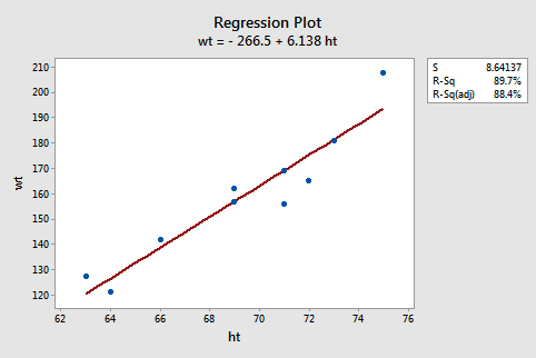
Now that we finished that investigation, you can just set aside the formulas for \(b_{0}\) and \(b_{1}\). Again, in practice, you are going to let statistical software, such as Minitab, find the least squares lines for you. We can obtain the estimated regression equation in two different places in Minitab. The following plot illustrates where you can find the least squares line (below the "Regression Plot" title).
The following Minitab output illustrates where you can find the least squares line (shaded below "Regression Equation") in Minitab's "standard regression analysis" output.
Analysis of Variance
Source | DF | SS | MS | F | P |
|---|---|---|---|---|---|
Constant | 1 | 5202.2 | 5202.2 | 69.67 | 0.000 |
Residual Error | 8 | 597.4 | 74.4 | ||
Total | 9 | 5799.6 |
Model Summary
S | R-sq | R-sq(adj) |
|---|---|---|
8.641 | 89.7% | 88.4% |
Regression Equation
wt =-267 + 6.14 ht
Coefficients
Predictor | Coef | SE Coef | T | P |
|---|---|---|---|---|
Constant | -266.53 | 51.03 | -5.22 | 0.001 |
height | 6.1376 | 0.7353 | 8.35 | 0.000 |
Note that the estimated values \(b_{0}\) and \(b_{1}\) also appear in a table under the columns labeled "Predictor" (the intercept \(b_{0}\) is always referred to as the "Constant" in Minitab) and "Coef" (for "Coefficients"). Also, note that the value we obtained by minimizing the sum of the squared prediction errors, 597.4, appears in the "Analysis of Variance" table appropriately in a row labeled "Residual Error" and under a column labeled "SS" (for "Sum of Squares").
Although we've learned how to obtain the "estimated regression coefficients" \(b_{0}\) and \(b_{1}\), we've not yet discussed what we learn from them. One thing they allow us to do is to predict future responses — one of the most common uses of an estimated regression line. This use is rather straightforward:
- A common use of the estimated regression line: \(\hat{y}_{i,wt}=-267+6.14 x_{i, ht}\)
- Predict (mean) weight of 66"-inch tall people: \(\hat{y}_{i, wt}=-267+6.14(66)=138.24\)
- Predict (mean) weight of 67"-inch tall people: \(\hat{y}_{i, wt}=-267+6.14(67)=144.38\)
Now, what does \(b_{0}\) tell us? The answer is obvious when you evaluate the estimated regression equation at x = 0. Here, it tells us that a person who is 0 inches tall is predicted to weigh -267 pounds! Clearly, this prediction is nonsense. This happened because we "extrapolated" beyond the "scope of the model" (the range of the x values). It is not meaningful to have a height of 0 inches, that is, the scope of the model does not include x = 0. So, here the intercept \(b_{0}\) is not meaningful. In general, if the "scope of the model" includes x = 0, then \(b_{0}\) is the predicted mean response when x = 0. Otherwise, \(b_{0}\) is not meaningful. There is more information about this in a blog post on the Minitab Website.
And, what does \(b_{1}\) tell us? The answer is obvious when you subtract the predicted weight of 66"-inch tall people from the predicted weight of 67"-inch tall people. We obtain 144.38 - 138.24 = 6.14 pounds - the value of \(b_{1}\). Here, it tells us that we predict the mean weight to increase by 6.14 pounds for every additional one-inch increase in height. In general, we can expect the mean response to increase or decrease by \(b_{1}\) units for every one-unit increase in x.